Forum Replies Created
-
AuthorReplies
-
January 26, 2022 at 6:01 pm in reply to: Does CasP Really Have a Theory of Value? Does It Need One? #247637
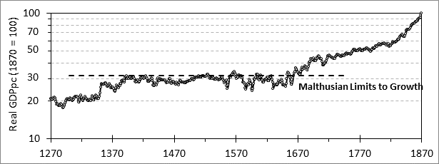
As a natural scientist, I come at this from a very different perspective. Below is a plot of per capita GDP (GDPpc) in England over six centuries. There was an initial rise in GDPpc around 1350 due to the Black Death, which reduced the number of people without reducing the amount of other factors of production (Land and Capital) resulting in a boost in labor productivity. There was a subsequent rise after 1370 due to the rise in real wages, which incented employers to optimize their use of increasingly expensive labor, resulting in a further rise of labor productivity. By 1400 these adjustments were complete and for 250 years GDPpc rose no further. This limit can be related to what is known as the Malthusian limits to growth which I will not go into here. What matters is how the profile was flat for a long time after 1400, but then started to rise in the last third of the 17th century, a trend that has continued to this day.
What happened? I define capitalism, in a phenomenological sense, as that which caused this trend change. I also note that the power a ruler could draw from the territory he ruled was directly dependent on GDPpc and on population, which also began to rise as agricultural productivity rose along with GDPpc. The result of this was the rulers of a small island in 1650 had, two centuries later, become the masters a globe-girdling empire encompassing a fourth of humanity. Clearly, this “capitalism” was a powerful “scale up tech” for rulers.
It was also clear that capitalism involved economic activity by private enterprise operating in a market milieu. But such activity had been going for millennia, in ancient Rome, medieval Islam and China, and elsewhere. Why didn’t this “capitalism” thing show up then? And what the hell was it? More on this later.
 January 24, 2022 at 9:36 pm in reply to: Military Spending and Economic Growth in the United States #247619
I don’t see the reason for the log transformation of the military spending. Why not plot the data w/0 transformation?
Scott: Why isn’t their real capital your real capital?
I think it probably is.
Equation 11 in the CasP stock model paper provides a link between the power index (PI) and Hussman’s HMI:
1. HMI = PI * residual
Now HMI is Market capitalization divided by gross value added (GVA). Divide the top and bottom by the number of shares (N) and you get index value divided by GVA/N. R is an easy-to-calucate approximation for GVA/N. Hence HMI is very similar to P/R, similar enough that any differences will be covered by the residual. So we can write
2. P/R = PI * residual
So P/R and PI are functionally equivalent.
Using the long-term S&P500 earnings growth rate since 1940 of 6% and the long term stock market return of 10% for the risk-adjusted expected return from stocks as r we get
3. K = 25 E, where E is the current *trend* earnings.
This is a theoretical result and must be multiplied by H to obtain the current realized value of K, as manifested in the stock market (P):
4. P = K * H = (25 * E) * H
Now E the *trend* value of E, not the spot value. Robert Shiller introduced the CAPE index in the late 1990’s. CAPE is simply the index divided by the trailing 10yr average of earnings. That is, it is the trend value of E five years on the past. Given a 6% trend growth rate we relate the E in equation 3 to Shiller’s E (Es) as follows:
5. E = 1.06^5 * Es = 1.33 * Es
Substituting eq 5 into eq 4 gives
6. P = 33 * Es * H
From eq 4 and 6 we obtain:
7. K = 33 * Es
Since CAPE is P / Es we can also write
8. K = 33 * P / CAPE
Here P is the index value and CAPE is the Shiller valuation measure. Equation 7 says the true amount of capital is what stock investors think it is (P) adjusted for the amount of hype (measured using CAPE) present in the market. That is, it is the quotient of the index price and a valuation tool. P/R is a valuation tool just like CAPE (that what I designed it to do). Hence using my conceptualization, I would estimate K as the quotient of P and P/R, that is R.
In other words, the CasP definition of capital and R are the functionally the same. What is different is the interpretation of what K (or R) means. In CasP K is a measure of power. In my treatment it is a cultural element. Since “power” in the sense used in CasP is social/political/economic/philosophical in nature, all of which are cultural entities, power itself is an expression of culture.
As I formulate it, political instability, rising inequality, financialization, and financial crisis arise due to cultural forces and are interrelated. From cliodynamics I obtained a relation between the political stress index (PSI) introduced by Jack Goldstone in the 1990’s and modified by Peter Turchin as follows (from chapter 2 of my book):
A simplified expression for PSI is given below:
(2.1) PSI=e^2/(EF*(1-EF))
Here EF refers to the fraction of GDP that goes to elites (a measure of inequality), and e is elite number as a fraction of population. A simple relation to model elite number is given below.
(2.2) de/dt = μo (((1-EF)o)/(1-EF) – 1)
Here μo, and (1-EF)0 are adjustable constants. Between equations 2.1 and 2.2 the value of PSI can be obtained directly from inequality. PSI leads directly to instability as measured by frequency of instances of social unrest (e.g. riots, strikes, mass shootings, uprisings etc). If unchecked by policy to reduce inequality, it typically leads to extreme unrest in the form of civil war, revolution, invasion, state collapse, coup, etc.)
From cultural evolution I obtained a model in which I can obtain inequality from historical top tax rate and labor power as measured by strike frequency. From Hyman Minsky and modeling by Steve Keen, I obtain a qualitative model for financial instability in which risk of financial crisis is measured by a financial instability index (FSI) analogous to PSI. This conceptualization adds financial/economic collapse as another possible outcome of times like we are in today.
All of this results from political policy choices made by elites (which in modern societies are capitalist elites, but before about 3 centuries ago were other kinds of elites). Policy is the application of power, which today is capitalist power, so my formulation is in the end the same as CasP.
Jon writes: I’m not sure what this measure tells us.
R provides a useful measure for capital. By this I means it serves a proxy for what “capital” needs to do. For example. capital, along with people and resources are a factor of production. Resources are consumed, their quantity does not affect output. If you double the size of the coal pile outside a power plant,you do not double the electrical output. On the other hand, capital and labor do affect the rate at which output is generated. Put a second generator in the power plant and you do increase the electrical output. Increase the number of installers and you can put more windows in. (We are having new windows installed and when asked how long it takes, they said all jobs take a day, they simply assign whatever number of installers necessary to get the job done in a day). Given these properties of workers and capital we expect that GDP should rise with population and have a special statistic, GDPpc, that we use to characterize growth in GDP independent of number of people. Thus, we should expect growth in GDPpc to reflect growth in capital, that is, capital accumulation.
The stock market is the capital market. Therefore, there should be a relation between the value of the stock market and the amount of capital. If we assume the S&P500 is a good proxy for the market as a whole, then the value of the index can serve as a measure of the amount of capital per share in the index.
R corresponds to both of these notions of what capital is.
[Jon] If the Standard Oil of New Jersey retained $20 million of net earnings in 1890, and if this $20 million was used to pay for drilling equipment, train companies, bribed politicians and what not, how much of this equipment, material or immaterial as the case may be, is still a “resource” in 2022?
None of it, as such. The money spent for the equipment is recovered by depreciation and so ceases to exist as a corporate asset on the books. The people trained/bribed are dead and so no trace of this still exists. The R created in 1890 was a resource in that year and measured at $20 million 1890 dollars ($540 million in 2020 dollars). The capital created by that investment is not associated with that equipment or training. It is the product of the increased sales (economic output) enabled by that investment. Those sales/output translate into increased income and a richer material environment resulting in a more complex culture that manifests as things like rising population-average IQ (Flynn effect).
[Jon] Your method suggests that all of it is, and you argue further that you know its quantity in ‘real terms’. My opinion is that you cannot know either.
The capital created by the investment in resources is preserved, the resources themselves are not. The former is part of the larger society, while the latter continues to belong to the company that made the original investment.
Jonathon writes “On an aggregate level, what capitalists buy with their profit is plant & equipment, or what economists call ‘real capital’ (buying other companies through mergers or acquisitions doesn’t alter the aggregate of what capitalists own, only redistributes it among them).”
But is it? In the trolley example the amount of capital connected with the trolley firms only manifested when they were destroyed. Similarly, when capitalists acquire other firms the price paid is typically more than the market value. The difference is known as goodwill. A significant fraction of of cumulative R consists of this goodwill that isn’t actually any sort of tangible thing, it certainly is not plant and equipment. It exists in the mind, but then so does culture (my take on the issue) or power (your take).
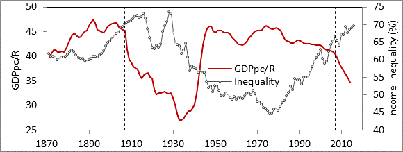
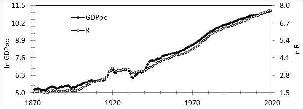
The key finding about R is that it works as a valuation tool (as does the power index). It also behaves like “that which when combined with people and resources produces output. This was shown by the correlation between GDPpc and R shown in my Jan 13 post. In fact, one can detrend per capita GDP by dividing by R. Two regimes can be seen. Over 1871-1907 and 1942-2006 this ratio ran in a fairly narrow range of 40-46. Between 1907 and 1942 and since 2006 the ratio declined dramatically indicating some sort of problem with how capitalism was operating. I call these periods capitalist crises.
I first saw this in 2010 and figured it was just an artifact. But after I learned about cliodynamics and secular cycles I was able to interpret it and wrote it up as a paper.
I’m going to have to respond to this. No, it’s not getting worse. When covid first showed up it was an entirely new disease. That’s a problem. We had a serious problem. In the US the crude death rate (by my own calculation–my wife and I are old and you can bet your ass we have been following it closely and doing calculations) was 1.5%. The R0 for the original strain was 2.5. Herd immunity is given by 1 – 1/R0, which was 0.6 for the original strain. So, 330 million pop x 0.6 x 0.015 = 3 million dead. This is a “back of the envelop calc, the real value would probably be lower. The number being floated then was 2 million (that was a *conservative* estimate). To avoid this, authorities decided to take century-old public health measures to slow the spread to give time for a vaccine to be developed. In May 2020 on a facebook group people asked me when I asserted we would have a vaccine by the end of the year why I was so sure this would happen. And I explained how this would happen (I retired in Feb 2021 from Pfizer after a 33 year career and knew folks who worked on the vaccine, which was produced in the town in which I live, so I know this).
By fall 2020 I was hoping for a “victory over Covid celebration to be held around Halloween time in 2021. This was based on my projection of a mass vaccination campaign to achieve a 60% vaccination level by the end of 3Q 2021. Then came Delta. The R0 for Delta is 6, for which herd immunity is >85%. That isn’t possible, so Covid in going to become endemic. We had already had 630K deaths. Mortality was still 1.5%. 15% of 330 million is 50 million. There were still about 140 million unvaccinated folks left of whom 90 million would get infected by Delta and 1.4 million would die, bringing total dead up to 2 million, one-third less than what we faced at the beginning. Added to these are those vaccinated who became infected by Covid.
Then came Omnicron. Here R0 is 10 and herd immunity 90%, suggesting 30 million will avoid infection. 37% of the population is unvaccinated, or 120 million. This means 90 million to get infected by ominicron. If omnicron is as deadly as delta then that means the same 1.4 million of extra deaths. But omnicron is *very* infectious and my wife and I (both in our sixties and with multiple risk factors) got it and it was like a cold. We know lots of young people who got the earlier versions of covid who did fine (and several older folks who did not, one of whom died). We were very scared of the earlier strains (I think justifiably so) but omnicron is different. I think it is milder and it has been reported as such. I will not have confirmatory data on that for another two weeks, based on my tracking, but I am optimistic.
Even so, worst case, the total death count we will see from this epidemic in the US will be significantly worse than what I projected at the beginning of the epidemic. It is not getting worse. It remains a very serious problem, but it has ALWAYS been a very serious problem for those who have been paying attention from the beginning.
I have been thinking about the problem of what is capital and capitalism. A problem I have with capitalism as power and capital as sabotage of industry is the startup problem. How can capitalist power be exerted when it is weak compared to other powers? And how can sabotaged industry come to dominate over non-sabotaged industry?
I prefer to think of capitalism as husbandry. A dairyman cares for his cattle so that he may extract their milk for his own purposes. A would-be dairyman can do the same by buying a breeding pair of cattle and then growing his own herd. Similarly, the capitalist husbands industry so that they may extract profit from that industry. A would-be capitalist can buy a bit of industry and grow it into a bigger industry. There is no start up problem.
So what is capital? Capital is what capitalists buy with their profits. This is a definition, it comes from Immanuel Wallerstein who defined capitalism as “the ceaseless accumulation of capital” an idea I believe originated with Marx (though I may be wrong here). Now one thing capitalists acquire a lot of is firms, through merger and acquisition deals. So let’s think of capital as whatever makes firms worth buying. Now CasP sees future earnings as what makes firms worth buying and that certainly is a valid way of looking at it. But the future profits are *not* necessarily connected with the thing that is being purchased. For example, the capital purchased when auto firms bought electric trolley firms was to be destroyed, there would be no future earnings coming from that specific capital. But doing this was expected to increase the profitability of their other capital (that related to autos). So, the auto firms *were* buying future earnings (i.e. capital) when they bought the trolleys, it just was capital that was never owned by the trolley companies. It had been *created* by the trolley companies and was real (this is why the auto firms had to *buy* it) but it did not ever belong to the trolley companies (because it was only fully manifested by the auto companies who bought them). Hence capital, though accumulated by individual firms, does not necessarily belong to them.
So rather than trying to measure capital in terms of an unknowable future stream of profits (that might not even materialize like that of the trolley companies before they were bought) why not measure it by the price (adjusted to constant dollars) that capitalists paid for it when they acquired it? That’s what R does.
I plotted out systemic fear and was looking at it. My understanding is system fear is associated with capital power. So I added labor power as proxied by strike frequency.
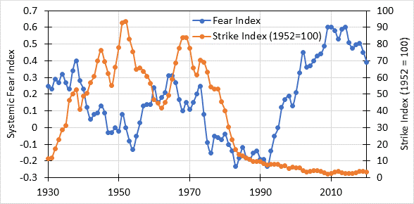
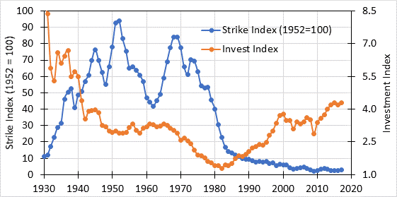
I would expect the two series to be inverses of each other, as in when capital power is high labor power is low and vice versa. This is the case for the measure I use for capital power, what I call the investment index, which is a ratio of the value of a portfolio of 50-50 stocks and bonds after taxes divided by a wage series. Here is investment index and labor power.
I looked over the stock market model paper. I also looks at the intro to the critique paper which provided a neat summary of the model:
A ‘power index,’ calculated by dividing the S&P 500 share price by the average wage rate from the late nineteenth century to the present, is tightly correlated with total returns for the S&P 500 twelve years later.
The power index is a detrended stock index, where a wage series is used for detrending. It provides a way to measure valuation levels that allows comparisons over time. There are lots of detrended indices, one of these is P/E, which Robert Shiller converted into his CAPE index that when presented to the Fed led to Greenspan’s “Irrational Exuberance” speech. Tobin’s Q is another example, as is Hussman’s valuation measure, and my own P/R.
In my own case, P/R reached its “irrational exuberance” moment in summer 1999 (see http://web.archive.org/web/20040406095317/http://csf.colorado.edu/authors/Alexander.Mike/Stanpor3a.html).
P/R gave a usable sell signal (I did sell in 1999 and it was a good move), whereas CAPE and Tobin’s Q were too early. P/R gave buy signals in July and Oct 2002 and in Nov 20 2008, which were also usable signals. It then gave sell signals in 2014 and 2020, which were wrong. All these are crude valuation-based predictions I used to test the validity of the valuation tool. What Hussman does is more sophisticated as he also uses a model based on technical analysis—which helps him avoid jumping the gun like I did.
We can use the power index to make predictions just as I did with P/R, when I was testing the concept. The close correspondence between the power index and Hussman’s valuation measure (see Fig 5 in model paper) to allow us to use 1% projected return (due to overvaluation) starting in 2013 (see Fig 4) to make short term predictions. The market in 2013 was at about 1600, while today it is 3000 points higher. According to the power index the 12-year return after 2013 are going to be low–in the 1% range. That is roughly similar to dividend yields which means the power index is forecasting that by 2025 we should see the index return to the neighborhood of 1600.
It will take about two years to get there, so we should see a big bear market beginning around the end of this year give or take six months, and probably an associated recession in 2023. How would that happened. I would guess it would reflect a growing sense that the Fed has dropped the ball on inflation, possibly because high inflation persists into the second half of this year, which is not what most people expect. A few years will tell the tale, lets’ see what happens. I hope it does, I sold out most of my stock positions back in 2013 based on Stock Cycle-based analysis, which is why I dropped work with long cycles in 2014 and started working with a new paradigm in my social science hobby.
First point, I interpreted cumulative retained earnings divided by a price index to mean (cumulative nominal retained earnings) divided by a price index, whereas it is cumulative (nominal retained earnings divided by a price index) or cumulative real retained earnings, they are different things.
Yes R contains past invested earnings, but not just invested in plant, equipment, raw material, knowledge, etc. 20 years ago most retained earnings were invested in stock of other companies through acquisitions and mergers. In terms of R what is being purchased is some other companies R which then gets added to your R. Tobin’s Q involves investment in the plant, equipment, raw material, knowledge, etc, but it failed as a valuation tool because it did not account for investment as mergers and acquisitions in which what is being bought is entirely intangible or in the case of stock buybacks, nothing. And yet nothing can be financially potent–look at cryptocurrencies. I used resources to separate R from the idea that it represented lant, equipment, raw material, knowledge, etc, because otherwise one can just use Tobin’s Q.
You write “capitalization, being the discounted value of risk-adjusted future earning, is theoretically independent of past profit.” But it’s not. Future earnings is not a thing theoretically because it is unknowable and so meaningless. Practically, for an index like the S&P500, it is pretty easy to predict. Plot log earnings over time and you get a pretty straight line so one can forecast future earnings by extrapolation of a fairly constant rate. The discount rate r is an arbitrary parameter that one can adjust to fit the data. This means that actual future earnings (EPS) divided by r can be represented by an adjustable parameter, k, times the present EPS (E) with which we can write eq 4 on p 189 as
P = (EPS / r) * H = k * E * H = E * (k * H) = E * (P/E)
In other words, one can represent the meaning of H using the index P/E, which varies widely over time, showing how hype changes. One of the factors affecting P/E or hype is the length of the amount of time the financial expansion has one on. The longer it does the greater the hype.
By introducing discounted future earnings you confuse the issue. What are the future earnings for cryptocurrencies or NFT? Yet these have prices and are a multitrillion dollar thing. The same thing could he said about internet stocks in the late 1990’s which is the environment in which I wrote Stock Cycles. Sure pets.com was worthless, but you couldn’t short that stock back then anymore than you can short Bitcoin today.
R represents an abstraction of the idea of “real capital.” Capital in the sense of plant, equipment, raw material, knowledge, etc should “work” for individual companies. R explicitly does not. This was shown by the stock prices tech companies with little (or no) earnings were fetching in the 1990’s. This was my take on what R meant in 2000:
**********************************
The underlying meaning of R is subtle. Some resources are physical assets such as plant and equipment, natural resources, or land that can be counted and which will show up on a balance sheet. Most of R resides in the brainpower of workers, however. A company in a declining industry will provide an environment that is less conducive to profit generation than a company in a rising industry. As a result the declining firm cannot attract and retain as many high-caliber employees, and they lose R as a result. Companies in rising industries gain increasing numbers of talented employees and gain R. In a way the new employees bring a little R with them when they join a company.New employees are not blank slates. Generally they can already communicate and process information. Often they already have specialized functions and knowledge bases. That is, they are an asset that produces a return, or they carry a little bit of R with them. Now where did they get this R? They got it as part of the cultural transmission they received from the previous generation. This quality of this transmission is a function of the richness of the cultural milieu in which the new worker was raised. The richer the milieu, the more R. As a result of the accumulation of past retained earnings, companies grow and pay increasing wages to workers, which makes society richer over time. The richer society provides an ever-improving cultural milieu in which the next generation is raised. Hence, successive generations have more R than the previous generations. For example, this rising R per worker is manifested by the tendency for population-average IQ scores to rise over time.
***************************This is a crude idea, but it contains the germ of the idea of capital as a cultural variant*, which is a non-economic thing, just as is your conception of capital as power.
*Theoretically capitalism is a social scale-up technology like religion or the state. The latter two increased group power (and so resistance to conquest) by increasing population size and/or social cohesion. Capitalism enhanced the amount of state power derived from a given population by boosting (taxable) economic output per person. This enhanced the ability of states/monarchs with this cultural attribute to contend with competitors leading to the spread of the capitalist cultural variant.
This is from Appendix A in Stock Cycles
For an index, R is given by:
A.1. R = R0 + sum of {(Ei-Di) · $CPIi } for i = 0 to i
Here Ei and Di are the earnings and dividend on the index at year i. The parameter $CPIi is the value of the historical dollar in year i in terms of 1999 dollars. The parameter R0 refers to the value of R in a basis year also expressed in 1999 dollars.
In the text R was introduced as follows:
In order to define the secular trends/stock cycles; it is useful to express the index value in terms of a parameter that is bounded (restricted to a range of values). An example of such a parameter is the price to earnings multiple or P/E. Stocks go up over time because earnings rise. The ratio P/E does not have to rise for stocks to go up, and P/E will generally remain within a range of values over very long periods of time. By using a bounded parameter like P/E, it should be possible to define stock cycles in terms of cyclical movements in the value of the parameter.
Since the cycles we wish to describe are quite long (28 years on average) P/E is not a good choice for this parameter. P/E fluctuates between high and low values more frequently than we would like for a 28-year cycle. The parameter I invented for stock cycles is P/R, the ratio of the index value (P) to business resources (R). Resources are simply the things (plant, equipment, technical knowledge, employee skills, market position etc.) available to the business owner to produce a profit. For a broad-based index, the value of R can be estimated as the sum of retained earnings in constant dollars as given by equation 3.1:
3.1 R = R0 + sum of rrEi for i = 0 to i
Here rrEi stands for the real retained earnings in year i. That is, it is the difference between what the stocks in the index earned collectively in year i and the dividends paid out in that year, expressed on a constant-dollar basis. R0 is the value of R in some basis year. For example, R for the S&P500 in fall 1999 was $950. Of this value, $880 represents the sum of rrE for 1999, 1998, 1997 all the way back to 1871 (all expressed in 1999 dollars). The remaining $70 represents the value of R in 1871 (R0).
P/R is just the S&P 500 index value divided by R. R tracks P for similar reasons as why E tracks P over time.
P/R is not a ratio of three indices. It is market price of a share divided by the equity value per share with equity calculated on a constant-dollar basis.
The idea is that when a firm retains profits, they are invested in non-money, or “real” objects, the prices of which rise with inflation.
For example, earnings on the S&P500 precursor in 1871 was 40 cents, while the dividend paid out was 26 cents. The index itself was $4.69. Retained earnings were $0.14. If we add this to the value of the index, we would say it was now “worth” 14 cents more or $4. 83. If we continue to 1910 this cumulative sum had risen to $9.93. More than half of the “worth” of the index was the result of profit generation (and retention) over the preceding 39 years. The index in 1910 was prices at $9.4. Here we see how the market price kept track with rising retained profits, or “equity”.
Continuing on for another forty years to 1950 the equity has now reached $24.05, while the index was now priced at $18.4, suggesting 1950 was a buying opportunity. And if we go another 40 years to 1990 equity has reached $193, while the market value was 335, suggesting the index should be sold as it was way overvalued. This was clearly wrong as subsequent market action revealed.
But if I do these same calculations by first putting the retained earnings for each year (and the initial index value) into constant dollar terms and then perform the same equity calculation I obtain the following values for 1910, 1950 and 1990: 9, 45.2, and 617. Here R correctly predicted that the index was very undervalued in both 1950 and 1990, which subsequent market action indicated was correct. Ten years later R has risen to 900, while the index now stood at 1427, way higher. Now R was indicating overvaluation. Old-school equity had been saying markers were overvalued for decades (and been wrong) while R was saying they were undervalued and had been right. Now it was the chance for R to be wrong. It wasn’t, future market action confirmed that assessment. By 201o R has reached 1572, while the index stood at 1139, suggesting undervaluation, which was confirmed by subsequent market action. But by 2019 R has reached 2400 while the index was now over 2900. R was no saying the market should fall in the future. And it did try to fall in March 2000 but then rose to dramatically higher levels because of Fed intervention. So R has now also been invalidated but that reflects external factors not accounted for in the R model.
P/R was invented as a tool for valuing the S&P 500 index. And it seems to have worked, giving correct assessments and allowing be to make a successful prediction back in 2000:
https://www.amazon.com/Stock-Cycles-Stocks-Markets-Twenty-ebook/dp/B0791LWTNK
As for point 3, this is best addressed by either reading my peer-reviewed paper on it
https://escholarship.org/uc/item/9x36913k
or sections 3.4 through 3.6 from my recent manuscript:
https://mikebert.neocities.org/Sec-cycle-book/secular%20cycles%20book-endnote.pdf
R is not cumulative retained earnings divided by a price index.
Back in the day, when a firm made a profit it paid out most of it to the owners, but retained a fraction that increased the assets held by the first by the amount retained. This made the company worth more by the amount retained (in theory). Over time the amount the firm was “worth” at time t was he amount it sold for at time zero plus the amount of profits retained over the intervening t years. This figure of cumulative retained profits is reported in a company’s statement of assets. Such information was private and sometimes kept secret for the public. Thus a stock market operator would try to sniff out hidden assets, acquire a position in the company and then publicize the assets, after which the price would rise to match the asset amount at which point the operator would sell. In other words, valuing a companies based on its net equity *worked* to reflect real prices, people made money this way and everyone knew this was how valuation worked. It was common knowledge that a company was worth its equity value, that is the amount of profits it had made (and kept) over time.
This stopped working when secular inflation became a thing and now equity or book value is pretty much meaningless.
R is this same equity calculation, except rather than use the nominal dollars I convert them to constant dollars and then sum them up. Unlike conventional equity, R continued to work for the stock indexed right up to 2000 when I used it to forecast a secular bear market in my first book Stock Cycles. It has only been in the last year or so that valuations have risen out of their historical range, making P/R no longer useful for valuing the index.
Although R can be calculated using financial data, it is *not* a financial quantity. It does not work for individual firms, but only for the index. There is no financial or economic reason for why this thing should show the same slope as the index, and indeed, it no longer seems to be doing so, but it did for nearly 150 years, for no apparent reason. It apparently measures something–it tracks per capita GDP over time, which is weird.
It is structured as a cumulative constant-dollar equity. Return on equity (ROE) is often seen as the same thing as return on capital (ROC). Based on this sense, R can be thought of as cumulative real capital or capital accumulation, which is consistent with the correlation between GDPpc and R. So years after coming up with R it occurred to me that perhaps R is a proxy for capital.
I did conceive of R as a cultural thing back then because there are several paragraphs in Stock Cycles that describe is as such, although culture was a fuzzy concept in my thinking at that time. Since learning about cultural evolution and cliodynamics and the mathematical apparatus for dealing with fuzzy things like culture more has fallen into place.
What you are doing with nomos and capital as power is along the same lines as my approach with capitalism as culture. But I would argue that power itself is a cultural manifestation and so ultimately falls under the capitalism as culture paradigm.
I have some quibbles with these definitions. Capital is defined financially, in terms of market capitalization. Capital has a second definition as the means of production. Put another way, we can say, the “resources employed by businessmen to produce a profit”. This is the definition I gave to what I called Business Resources or R. R is also defined as the cumulative sum of retained earnings on the S&P 500 in constant dollars plus the real value of the index in 1871, when data becomes available. To the extent that the S&P500 index is representative of the economy as a whole, R can function as a proxy for the amount of real capital in the economy. This figure shows a plot of R and per capita GDP since 1871.
With R representing the “real capital”, and the price of the index representing “financial capital” one can relate the two in terms of the ratio P/R. This is the financial value for capital compared to real value for capital and could be used as a tool for determining how over or under valued the market is at any point in time. Such a plot shows range-bound behavior for two centuries.
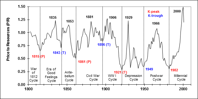
In recent years P/R has risen above its previous high in 2000 which is either indicative of a massive bubble that will correct downward at some point, or an entirely new mode of capitalist operation. I note that the concept of capital as R is essentially the same as the Marxian notion of capital as the means of production.
Now a main point of my book is that capitalism is a cultural construct (like everything else in the human world) and evolves just like other kinds of culture. So on can apply the methods of cultural evolution as developed by Boyd, Richerson, Henrich, and others to evolution of capitalism. I use a very simplified model involving two kinds of capitalism, shareholder primacy (SP) and stakeholder capitalism (SC). The first uses the financial definition of capitalism, while the second uses the Marxian one. Which one you get depends on the economic and business environment. An environment of low marginal tax rates on income, low tariffs, inflation control using interest rates, legal stock buybacks, such as we have had since the 1970’s, selects for the SP variant. An environment of high marginal tax rates, high tariffs, fiscal inflationary control, and illegal stock buybacks selects for the SC variant. I use a measure of income inequality (top 1% income share) as a proxy for the amount of SP capitalism. Using a cultural evolutionary model I got from Boyd and Richerson’s primer on the topic I obtain this result when fitting inequality data to the model
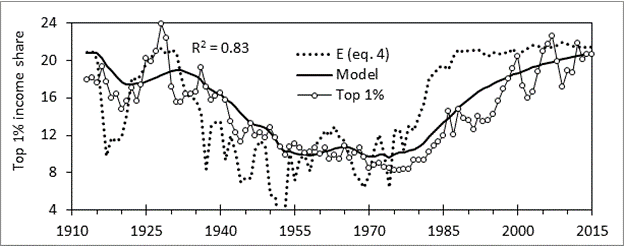
Here “E” refers to the environment in which capitalist evolution is taking place. It is a function of policy set by the state: here represented as a linear function of top tax rate and labor power (measured by strike frequency). The heavy black line is the cultural evolutionary response to the changing environment E, and the open symbols is top 1% income share used as a proxy for amount of SP culture versus SC culture. -
AuthorReplies
