Debunking the ‘Productivity-Pay Gap’
November 9, 2020
Originally published on Economics from the Top Down
Blair Fix
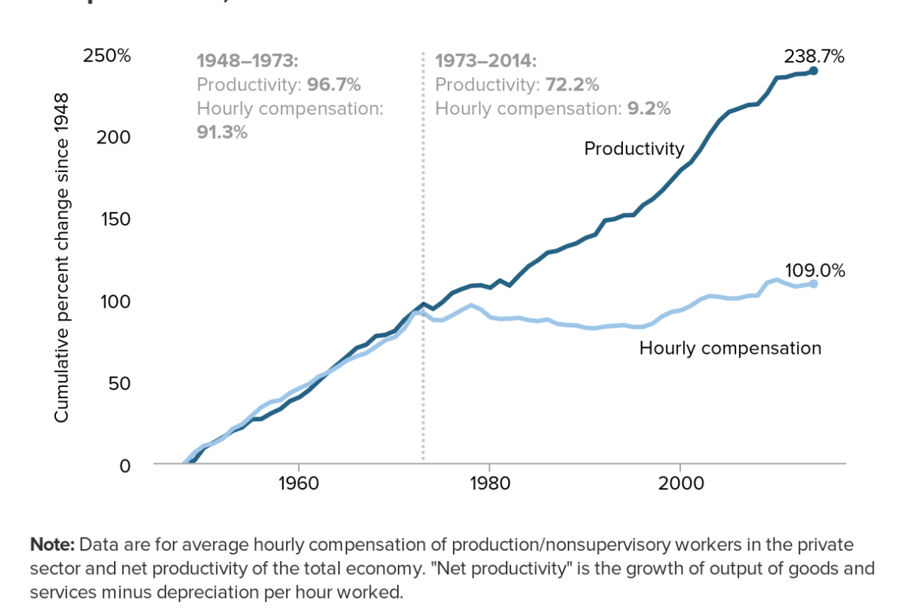
Have you heard of the ‘productivity-pay gap’? It’s the (apparently) growing gap between the productivity of US workers and their pay. Here’s what it looks like:

Figure 1: The Productivity-Pay Gap. Source: Economic Policy Institute.
In this post, I debunk the ‘productivity-pay gap’ by showing that it has nothing to do with productivity. The reason is simple. Although economists claim to measure ‘productivity’, their measure is actually income relabelled.
As a result, the ‘productivity-pay gap’ isn’t what it appears. It claims to be a gap between productivity and wages. But it’s not. It’s really a gap between two types of income — (1) the wages of workers and (2) the average hourly income of all Americans. This gap is an important measure of inequality. But it has nothing to do with ‘productivity’.
How economists measure productivity
To understand the problem with the ‘productivity-pay gap’, we first need to understand how economists measure productivity. Economists define ‘labor productivity’ as the economic output per unit of labor input:
To use this equation, we’ll start with a simple example. Suppose we want to measure the productivity of two corn farmers, Alice and Bob. After working for an hour, Alice harvests 1 ton of corn. During the same time, Bob harvests 5 tons of corn. Using the equation above, we find that Bob is 5 times more productive than Alice: [1]
Alice’s productivity: 1 ton of corn per hour
Bob’s productivity: 5 tons of corn per hour
When there’s only one commodity, measuring productivity is simple. But what if we have multiple commodities? In this case, we can’t just count commodities, because they have different ‘natural units’ (apples and oranges, as they say). Instead, we have to ‘aggregate’ our commodities using a common unit of measure.
To aggregate economic output, economists use prices as the common unit. They define ‘output’ as the sum of the quantity of each commodity multiplied by its price:
So if Alice sold 1 ton of corn at $100 per ton, her ‘output’ would be:
Alice’s output: 1 ton of corn × $100 per ton = $100
Likewise, if Bob sold 5 tons of potatoes at $50 per ton, his ‘output’ would be:
Bob’s output: 5 tons of potatoes × $50 per ton = $250
Using prices to aggregate output seems innocent enough. But when we look deeper, we find two big problems:
- ‘Productivity’ becomes equivalent to average hourly income.
- ‘Productivity’ becomes ambiguous because its units (prices) are unstable.
‘Productivity’ is hourly income relabelled
By choosing prices to aggregate output, economists make ‘productivity’ equivalent to average hourly income. Here’s how it happens.
Economists measure ‘output’ as the sum of the quantity of each commodity multiplied by its price. But this is precisely the formula for gross income (i.e. sales). To measure gross income, we multiply the quantity of each commodity sold by its price:
To find ‘productivity’, we then divide ‘output’ (gross income) by the number of labor hours worked:
When we do so, we find that ‘productivity’ is equivalent to average hourly income:
So economists’ measure of ‘productivity’ is really just income relabelled. The result is that any relation between ‘productivity’ and wages is tautological — it follows from the definition of productivity.
Ambiguous ‘productivity’
In addition to making ‘productivity’ equivalent to average hourly income, using prices to measure ‘output’ also makes ‘productivity’ ambiguous. This seems odd at first. How can ‘productivity’ be ambiguous when income is always well-defined?
The answer has to do with prices.
We expect prices to play an important role in shaping income. Suppose I’m an apple farmer who sells the same number of apples each year. If the price of apples doubles, my income doubles. That’s how prices work.
If ‘output’ is equivalent to income, it seems that my ‘output’ (of apples) has also doubled. But here economists protest. Your apparent change in ‘output’, they say, was caused by a change in price. To find the ‘true’ change in output, you need to hold prices constant. When you do, you’ll find that your ‘output’ remains the same.
On the face of it, this ‘adjustment’ for price change seems reasonable. But it actually leads to a measurement quagmire. To see this quagmire, we’ll return to Alice and Bob.
Suppose that Alice grows 1 ton of corn and 5 tons of potatoes. Bob grows 5 tons of corn and 1 ton of potatoes. Whose output is greater? The answer is ambiguous — it depends on prices.
Suppose that corn sells for $100 per ton and potatoes sell for $20 per ton. We find that Bob’s output is about 250% greater than Alice’s:
Alice’s Output: 1 ton corn × $100 per ton + 5 tons potatoes × $20 per ton = $200
Bob’s Output: 5 tons corn × $100 per ton + 1 ton potatoes × $20 per ton = $520
Now suppose that corn sells for $20 per ton and potatoes sell for $100 per ton. We now find that Bob’s output is about 60% less than Alice’s:
Alice’s Output: 1 ton corn × $20 per ton + 5 tons potatoes × $100 per ton = $520
Bob’s Output: 5 tons corn × $20 per ton + 1 ton potatoes × $100 per ton = $200
What’s going on here? When we aggregate output using prices, these prices determine the relative weighting given to corn and potatoes. When this weighting changes, the measurement of ‘output’ changes.
As a result, our measure of ‘output’ depends on the particular prices we choose to hold constant. This is a big problem. It means that standard measures of productivity are inherently ambiguous. (For more details about this ambiguity, see my work with Jonathan Nitzan and Shimshon Bichler and with Erald Kolasi.)
To summarize, using prices to aggregate ‘output’ leads to bizarre problems. On the one hand, it causes ‘productivity’ to be equivalent to average hourly income. This means that any connection between ‘productivity’ and wages is circular. On the other hand, the same decision causes ‘productivity’ to be ambiguous. Our measure of ‘productivity’ depends on arbitrary choices about how to adjust for price change. As a result, productivity trends (like the one in Figure 1) are riddled with uncertainty.
Dissecting the ‘productivity-pay gap’
Now that you understand the problems with how economists measure productivity, let’s return to the ‘productivity-pay gap’. I’m going to dissect the evidence in Figure 1.
This chart comes from the Economic Policy Institute (EPI). By dissecting it, I don’t mean to pick on the EPI authors. They use methods that are standard in economics. Instead, I want to show why these standard methods are flawed.
We’ll start with how the EPI measures productivity. They write:
“Net productivity” [of workers] is the growth of output of goods and services less depreciation per hour worked.
To non-economists, this sounds like the EPI is measuring some physical quantity of output. But they’re not. Instead, the “output of goods and services” is economists’ code for the value of goods and services, as measured by Gross Domestic Product (GDP). ‘Depreciation’ is code for the financial depreciation of capital.
When we subtract capital depreciation from GDP, we get something called ‘Net Domestic Product’:
So the EPI defines ‘economic output’ in terms of Net Domestic Product.
Now here’s the rub. The national accounts are based on the principles of double-entry bookkeeping. This means that for every sale there is a corresponding income. So when you build a house and sell it for $1 million, you record the sale in one ledger as ‘output’. On the opposite ledger, you record the same sale as ‘income’. So ‘output’ is formally equivalent to income.
In the national accounts, Net Domestic Product is the sales side of the ledger, recorded as ‘output’. It’s equivalent to the income side of the ledger, which we call ‘National Income’ — the income of all individuals in the country:
I’ve put the ‘≈’ here to mean ‘almost equivalent’. There are some small differences between Net Domestic Product and National Income (some business taxes, for instance). But in practice, the two quantities are nearly identical, as shown in Figure 2.
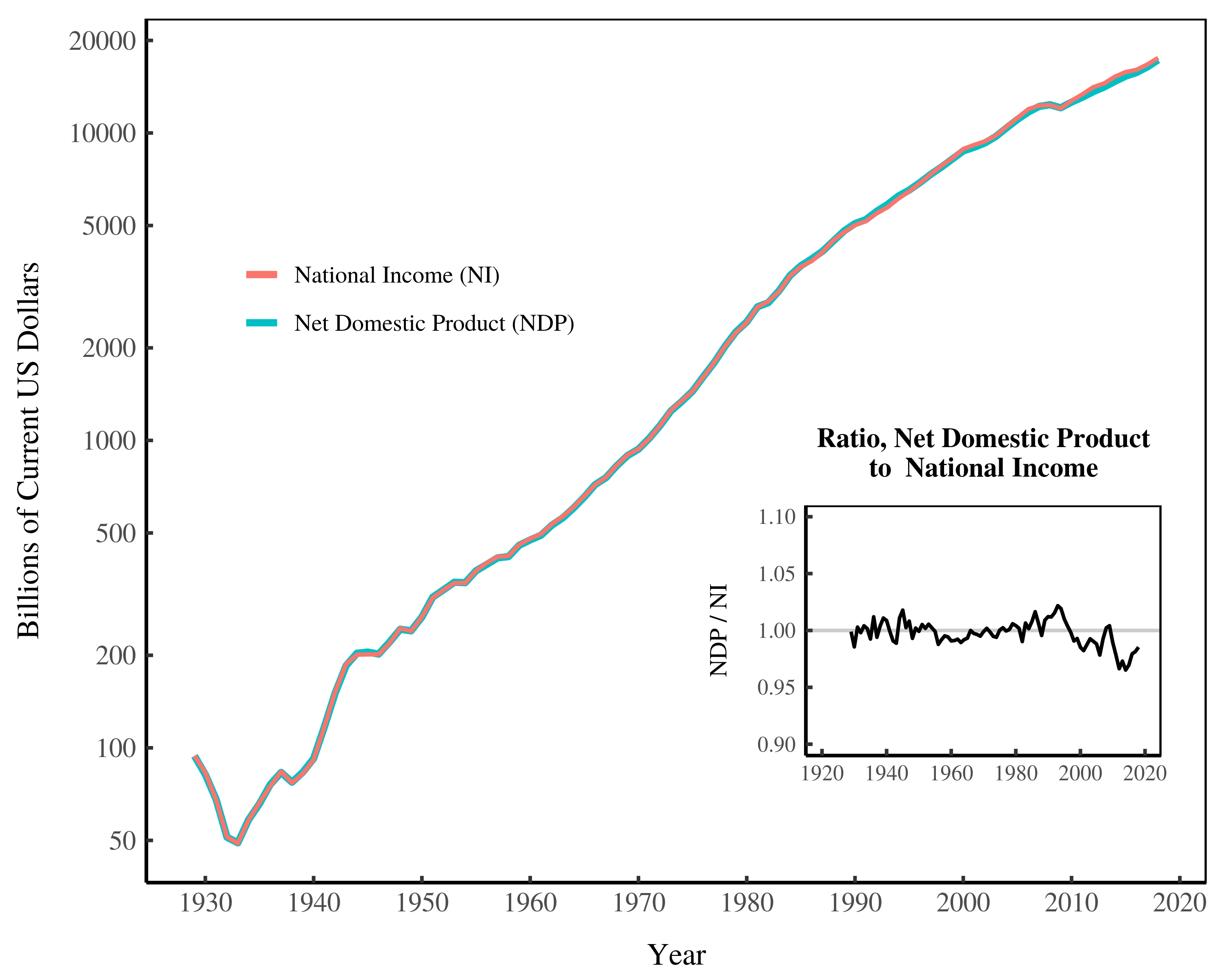
Figure 2: US Net Domestic Product And National Income. Data is from the Bureau of Economic Analysis Table 1.7.5.
To calculate workers ‘productivity’, the EPI divides Net Domestic Product by the number of labor hours worked:
But this is equivalent to dividing National Income by the number of labor hours worked:
When we divide National Income by total labor hours, we’re actually measuring average hourly income. So the EPI’s measure of ‘productivity’ is identical to average hourly income:
Given this equivalence, any connection between ‘productivity’ and average hourly income isn’t surprising. It’s a tautology.
How can wages diverge from ‘productivity’?
If productivity is equivalent to average hourly income, how can wages diverge from ‘productivity’? In other words, how can the ‘productivity-pay gap’ exist?
Let me explain.
‘Productivity’ (as measured by the EPI) is equivalent to the average hourly income of all US earners. Since average income can’t diverge from itself, average income and ‘productivity’ can’t diverge. However, if we select a subpopulation of US citizens, their income can diverge from the average. This is just a mathematical truism. If I select a non-random sample from a population, the properties of this sample need not match the properties of the whole population.
To make this thinking concrete, suppose we select only CEOs. Must CEO income track with the national average? The answer is no. CEOs are a unique subpopulation, so their income can diverge from the national average. And as you probably know, CEO income has done just that. Over the last 40 years, the income of US CEOs has grown drastically relative to average income.
Wages of production workers
In Figure 1, the EPI studies the wages of ‘production/nonsupervisory workers’. Because these workers are a subpopulation of the US, their income can (and does) diverge from the national average. Over the last 40 years, the wages of production workers have declined relative to the average hourly income.
This decline, however, has nothing to do with productivity. Instead, it owes to a redistribution of income — a redistribution that has two parts. First, the labor share of national income has declined over the last 40 years. Second, over the same period, US wages and salaries have become increasingly unequal.
The declining labor share of income
In the national accounts, there are two basic types of income. If you earn income from property, you earn ‘capitalist income’. If you earn income from wages and salaries, you earn ‘labor income’. The two types of income sum to National Income:
If we select only ‘laborers’, it’s possible for the average hourly income of this subpopulation to diverge from the average income of the population. For instance, if capitalist income grows relative to workers’ income, it pulls up the average income. This causes a gap between the wages of workers and the hourly income of the whole population.
Looking back at Figure 1, we see that the ‘productivity-pay gap’ emerges after 1970. Not surprisingly, it’s around this time that the labor share of US income began to drop:
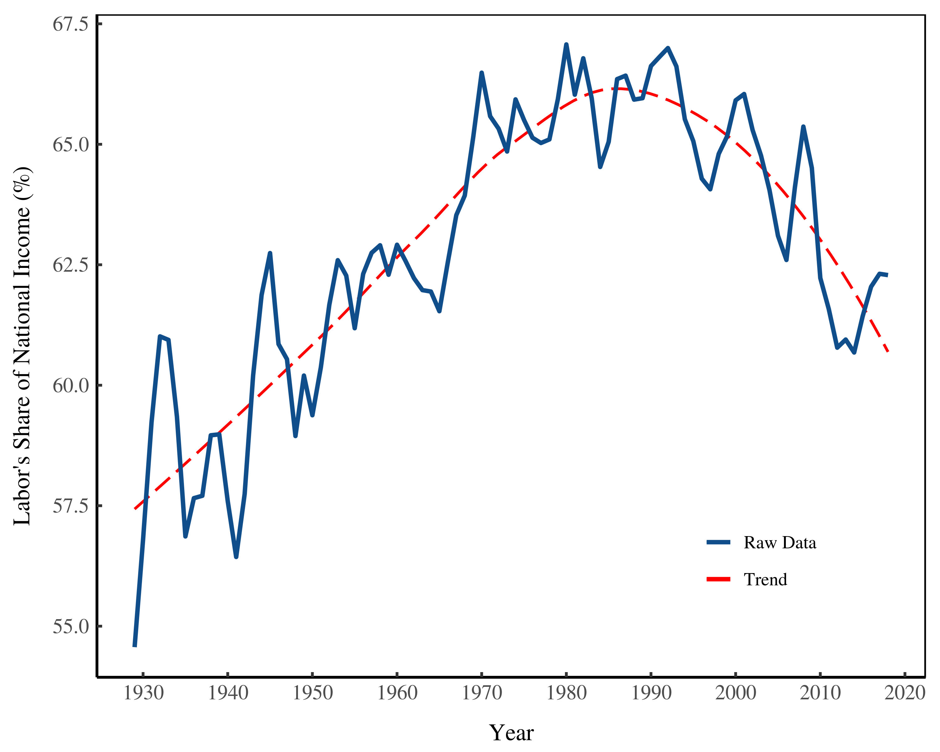
Figure 3: Labor’s Share of US National Income. Data is from the Bureau of Economic Analysis Table 1.12. Labor’s share is calculated as the ‘compensation of employees’ as a fraction of national income.
This decline of labor’s share of income is partly why the EPI finds a ‘productivity-pay gap’. Remember that ‘productivity’ (as measured by the EPI) is equivalent to the average hourly income in the US. Since 1970, US workers have received a declining share of this income. Consequently, their wages have declined relative to the average US income.
The growing inequality of labor income
The other reason that the EPI finds a ‘productivity-pay gap’ is because US wages and salaries have become increasingly unequal. Since 1970, the income share of the top 1% of wage/salary earners has grown steadily:
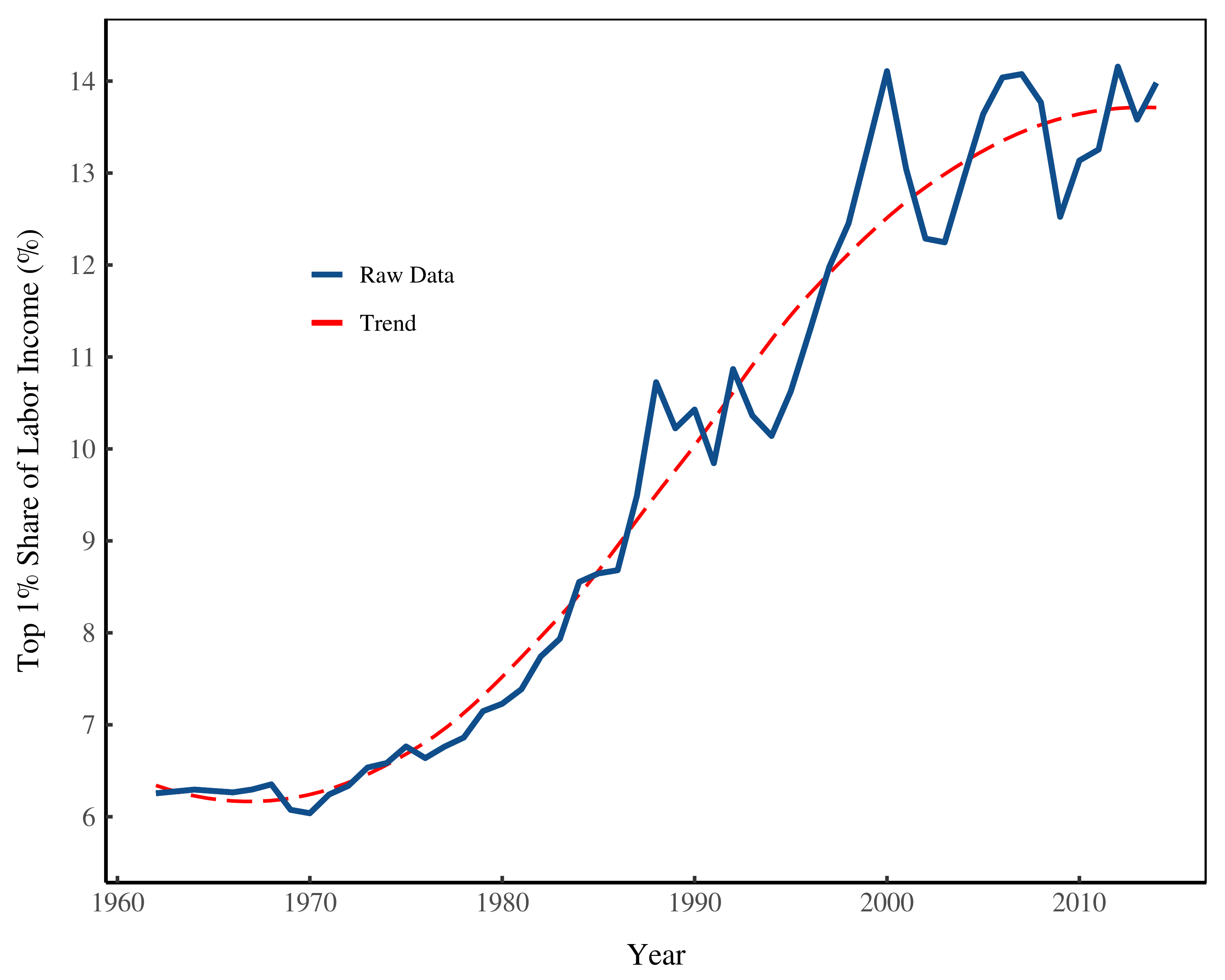
Figure 4: Top 1% of Wage/Salary Earners, Share of US Labor Income Data is from the World Inequality Database (average of series flinc and plinc).
It may not be clear how wage inequality would affect the relative income of production workers. To help understand, we’ll divide labor income into two parts:
Suppose that the income of non-production workers increases relative to the income of production workers. This increase pulls up the average labor income, causing it to outpace the average income of production workers. Still, it’s not clear how this redistribution relates to wage inequality.
This is where hierarchy comes in.
I propose that ‘production workers’ occupy the bottom two ranks in firm hierarchies. The bottom rank consists of ‘shop floor’ workers. The second rank consists of ‘working supervisors’. Everyone in ranks three and above is a ‘non-production worker’ (i.e. manager).

Figure 5: Production workers in a hierarchy. Production workers (blue) occupy the bottom two ranks in a hierarchy. The first rank contains ‘shop floor’ workers. The second rank contains ‘working supervisors’. Ranks three and above are ‘managers’.
In this simple model, ‘production workers’ make up about 77% of total employment. That’s not far from the actual US figure of 82%.

Figure 6: Production workers’ share of US private employment. Data is from the Bureau of Labor Statistics, series CES0500000001 and CES0500000006.
What does our hierarchy model tell us about the income of production workers? In hierarchies income increases steeply with hierarchical rank. (I review the evidence here and here.) So if production workers occupy the bottom of the corporate hierarchy, they should also occupy the bottom of the income distribution.
Let’s suppose that production workers occupy the bottom 80% of US labor incomes. If labor income inequality increases, we expect the relative income of production workers to decline.
Figure 7 shows a simple model of what this might look like. Here I’ve defined ‘production workers’ as everyone in the bottom 80% of a hypothetical distribution of income. I then calculate the average income of these production workers and compare it to the average income in the whole population.

Figure 7: A model of the relative income of production workers. Here I model ‘production workers’ as the bottom 80% of earners in the population. As inequality (measured by the top 1% share of income) grows, the average income of production workers declines relative to the average income of the population. For the math people, I’ve modeled the distribution of income with a lognormal distribution.
Because production workers are at the bottom of the income distribution, we expect their income to be below the population average. (That’s why the y-axis values in Figure 7 are below 100%.) But just how far below depends on income inequality.
As we increase inequality in the population (shown on the horizontal axis in Figure 7) the relative income of production workers declines. When inequality is minimal, production workers’ relative income approaches the population average. When inequality is extreme, production workers’ relative income approaches zero.
In Figure 7, the vertical red lines show the US top 1% share of labor income in 1970 and 2012. Given this growing inequality, our model predicts that the relative income of production workers should drop by about 50%. This is on par with the pay gap shown in Figure 1.
In short, the growing inequality of labor income can explain a large part of the apparent ‘productivity-pay gap’. Again, this gap isn’t about productivity. It’s about the declining relative income of production workers.
The price-index problem
While most of the apparent ‘productivity-pay gap’ has been caused by income redistribution, part of this gap is caused by price index shenanigans. In Figure 1, the EPI uses two different price indexes to ‘adjust’ for inflation.
To understand the problems with the EPI’s method, we need to backtrack a bit. I’ve already noted that ‘productivity’ is equivalent to average hourly income. But this wasn’t quite correct. ‘Productivity’ is equivalent to real average hourly income:
Unlike ‘nominal’ income, ‘real’ income adjusts for inflation. To get ‘real’ income, we divide ‘nominal’ income by a price index — a measure of average price change:
There are many different types of price indexes. Some track a few commodities. Others track many commodities. Because price change varies wildly between commodities, different price indexes can vary wildly.
Here’s where the EPI errors. It uses the (implicit) Net Domestic Product deflator to measure ‘productivity’ (i.e. real average income per hour). But it uses the Consumer Price Index (CPI) to measure the ‘real’ wage of production workers.
This is a problem. The two price indexes have diverged since 1970 — the very period where the EPI finds a growing ‘productivity-pay gap’. Here’s what the divergence looks like:
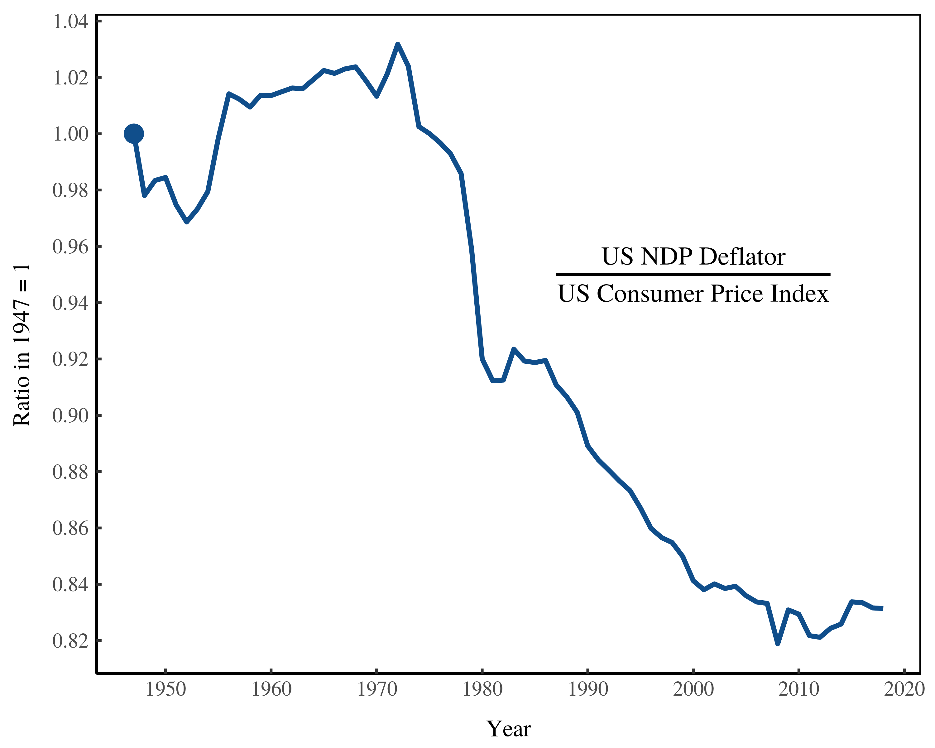
Figure 8: The US Net Domestic Product deflator relative to the Consumer Price Index. CPI data is from Federal Reserve Economic Data, series CPIAUCSL. The implicit NDP deflator data is from BEA Table 1.17.6 (the ratio of nominal NDP to real NDP).
To put this in perspective, the EPI’s method is like using different price indexes to compare the ‘real’ income of two people. Suppose Alice and Bob both start out with $100. Over 40 years, both of their incomes grow to $200. We then use the NDP deflator to find Alice’s real income. But we use the CPI to find Bob’s real income. Although their nominal incomes are identical, we find that Alice’s real income outpaced Bob’s by 20%.
The crime here is that we don’t need price indexes to compare incomes. We can compare Alice and Bob’s incomes directly. Similarly, the EPI could have compared the nominal income of production workers directly to the nominal hourly income in the US.
The declining relative income of workers
The problem with the ‘productivity-pay gap’ is that it proclaims to be something it’s not. It’s not a gap between workers’ productivity and their income. Instead, it shows the declining relative income of workers.
The best way to look at this decline is to measure the relative income of production workers:
Figure 9 shows this relative income over the last 50 years. In 1964, US production workers earned 60% of the average hourly US income. By 2015, this declined to 35%.
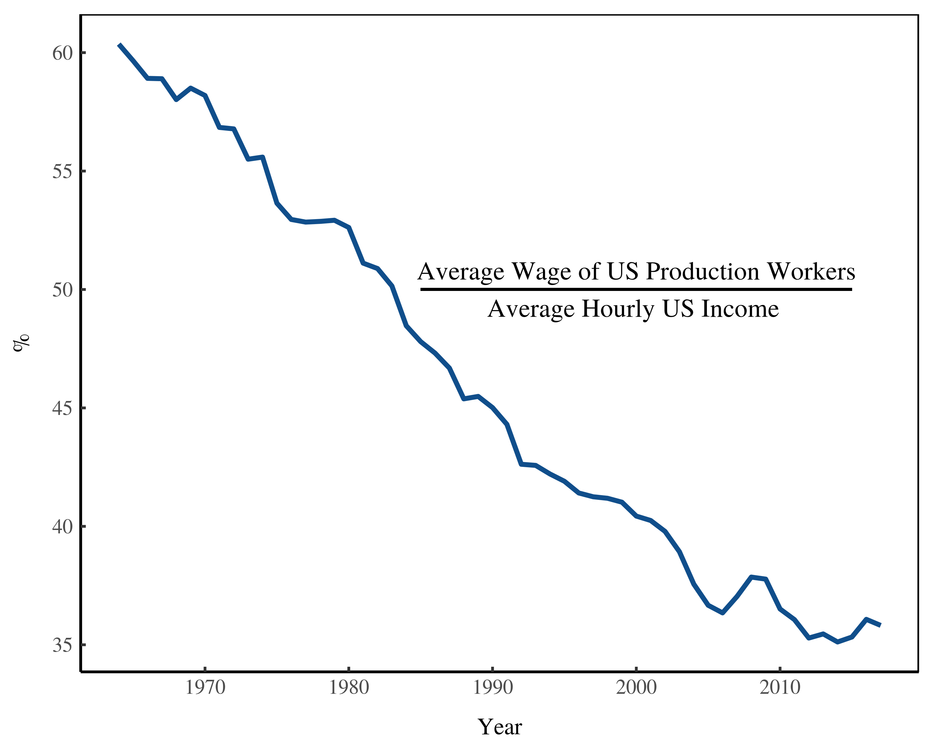
Figure 9: The relative income of US production workers. Average hourly earnings of production workers is from FRED series AHETPI. Average hourly US income is calculated by dividing National Income (BEA Table 1.7.5) by the number of labor hours worked by US persons engaged in production (FRED series EMPENGUSA148NRUG × series AVHWPEUSA065NRUG).
What’s important here is that we haven’t dressed up income as ‘productivity’. We’re explicitly comparing two types of income — the income of production workers relative to the national average.
The relative income of production workers has nothing to do with ‘productivity’. It’s actually a measure of income inequality. As shown in Figure 10, production workers’ relative income correlates strongly with the income share of the top 1%. As income inequality increases, the relative income of production workers decreases.
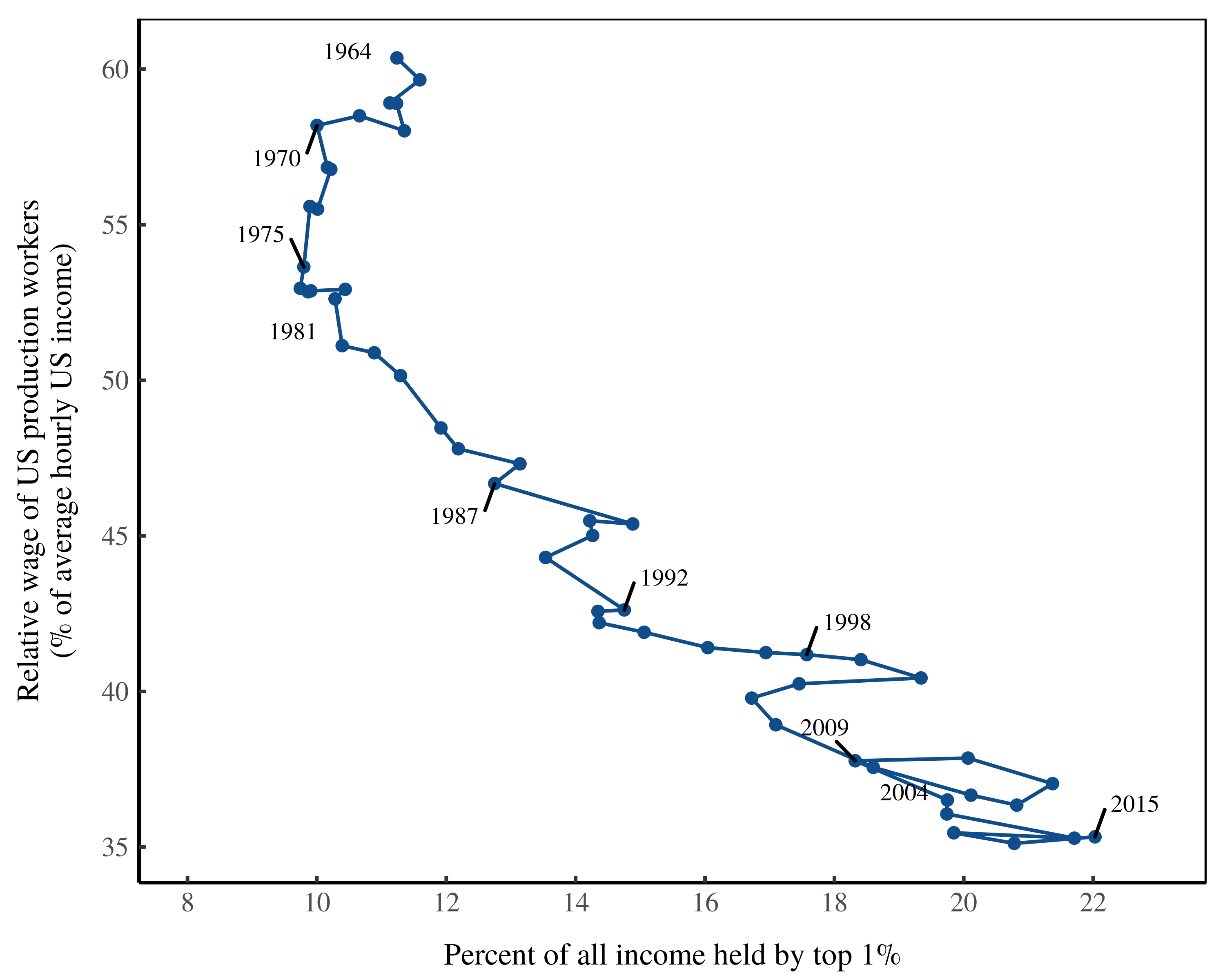
Figure 10: The relative wages of production workers decline as US inequality increases. For the sources for relative wages, see Figure 8. Data for the top 1% share of income comes from the World Inequality Database.
Is ‘productivity’ still increasing?
The tale told by the ‘productivity-pay gap’ (Figure 1) is that workers’ productivity has increased steadily but wages have not. This is a powerful piece of propaganda. It says to workers “look, the tide has risen, but it didn’t lift your boat”.
The problem, though, is that it’s not clear that the tide has actually risen. We can say for certain that workers relative wages have declined (Figure 9). But what about their productivity? Has it gone up as Figure 1 suggests?
To believe the ‘productivity’ trends in Figure 1, you have to put on a brave face. You have to believe that the myriad of subjective decisions made by statistical agencies (reviewed here) are the ‘correct’ decisions. You have to believe that prices ‘reveal’ utility, and that monetary income is the same as economic ‘output’.
I, for one, don’t believe these things. Consequently, I treat official measures of ‘productivity’ as garbage.
How should we measure productivity? It depends on what we think the economy ‘does’. Personally, I like the view taken by atmospheric scientist Tim Garrett. He treats the economy as a heat engine. Garrett uses the analogy of a growing child. It takes energy to maintain the child’s body. And if the child is to grow, it needs to consume increasing amounts of energy. The same is true of the economy.
When you think this way, you realize that ‘useful work’ (the amount of energy put to an end use) is a good indicator of economic output. I propose that we treat useful work per labor as an alternative measure of labor productivity.
How does this alternative measure compare with the standard measure of productivity? Figure 11 shows a comparison. Here I use real GDP per labor hour as the standard measure of productivity. I contrast this with Benjamin Warr and Robert Ayres’ estimate for useful work per labor hour.
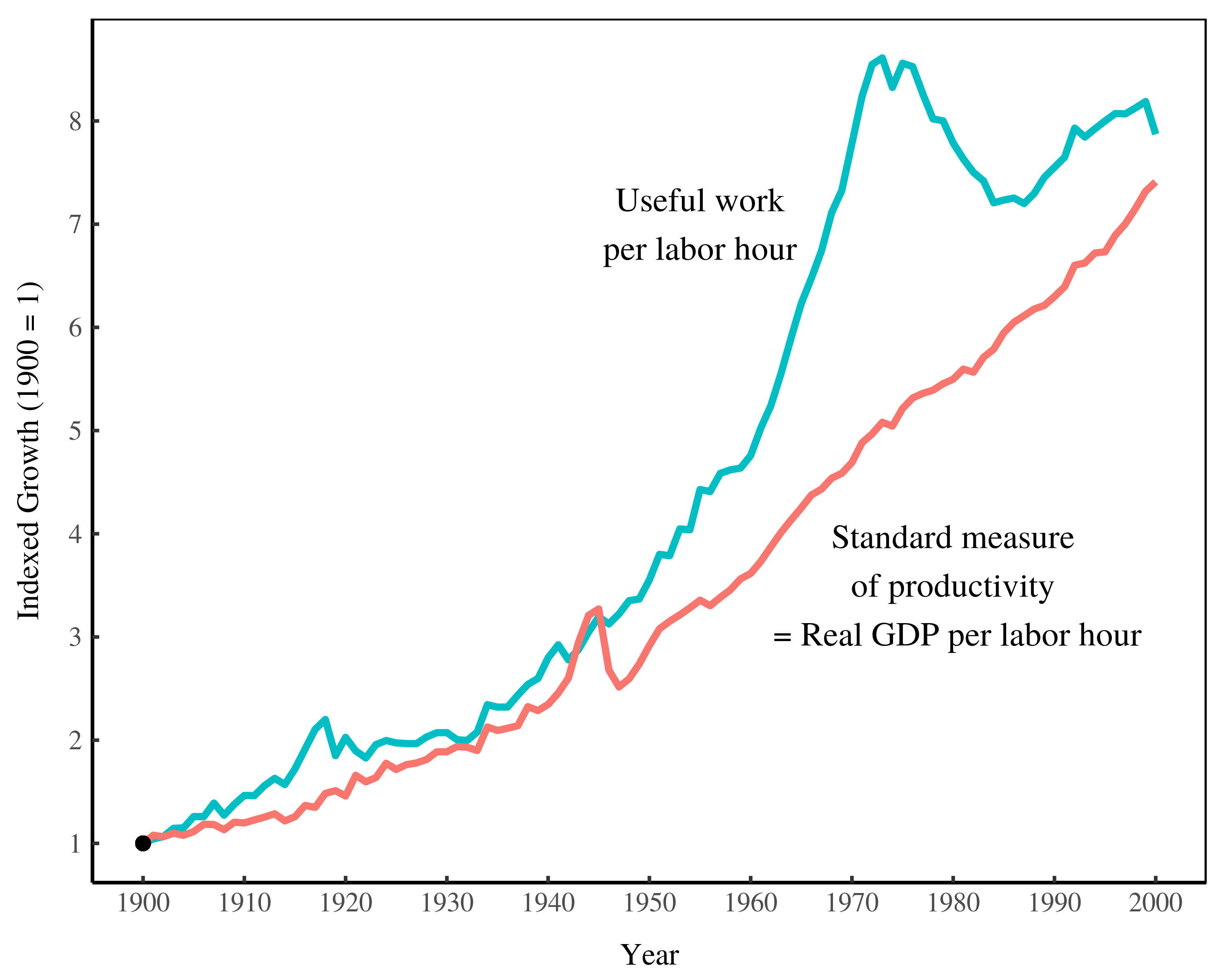
Figure 11: How a physical measure of US productivity compares to the official measure of productivity. Data is from Benjamin Warr’s REXS Database.
It’s not hard to spot the difference between the two series. The standard measure of productivity tells a tale of steady growth. In contrast, our physical measure suggests that productivity has stagnated since 1970. Interestingly, this is the period when the relative wages of production workers began to decline (i.e. when the apparent ‘productivity-pay gap’ appears).
Here’s an interesting question. Is the stagnation in useful work output related to the decline of workers’ wages? Biophysical economist Carey King thinks so. He recently built a model to investigate this connection.
The important point is that it’s far from clear that US productivity has increased steadily over the 20th century. In energetic terms, productivity has stagnated since 1970. I, for one, think that this physical measure of productivity is far more meaningful than the official measure. ‘Useful work’ is based on the laws of thermodynamics. The standard measure of productivity, in contrast, is based on the dubious assumptions of neoclassical economics.
The productivity problem
‘Productivity’ is used by both major schools of economic thought. Neoclassical economists use productivity to claim that the distribution of income is just. They argue that in a competitive economy, workers get what they produce. Marxists, in contrast, use productivity to claim that the distribution of income is unjust. They argue that in a capitalist economy, workers receive less than they produce (because capitalists extract a surplus).
What’s interesting is that these two opposing theories commit the same sin. They define productivity in terms of income. Neoclassical economists do so explicitly, as I’ve described in this post. Marxists do so implicitly because they haven’t developed their own system of national accounts. Instead, Marxists who do empirical work use neoclassical measures of productivity (As an example, see this fascinating exchange between Paul Cockshott, Shimshon Bichler and Jonathan Nitzan.)
The result of this circular definition is that the analysis of productivity is a sleight of hand. ‘Productivity’ is just income relabelled.
The ‘productivity-pay gap’ is a textbook example of this relabelling. It claims to show a growing gap between what workers ‘produce’ and what they get paid. But workers’ ‘productivity’ is actually measured in terms of income — the average hourly income.
This relabelling of income gives the analysis ideological potency. Instead of saying that workers’ relative wages have declined, it says that workers don’t get paid what they produce. The latter, as Marx long ago realized, is far more potent propaganda.
Productivity propaganda cuts both ways
The problem with productivity propaganda is that it cuts both ways. The EPI uses income to measure ‘productivity’ at the national level. But why stop there? Why not equate income and productivity at the sector level, or at the individual level? Curiously, the EPI warns against doing so (see the technical appendix here).
The problem is that the more finely we equate income with productivity, the more we’ll find that everyone ‘gets what they produce’. This is because as we study smaller and smaller groups, we remove the possibility of sampling subgroups whose income diverges from the group’s average income.
As a progressive think tank, the EPI wants to show that workers do not get paid what they produce. So it warns against equating income and productivity at the sector and individual level.
The problem is that the EPI wants to have its cake and eat it too. It wants to equate productivity with income when the results suit it — when the analysis shows a productivity-pay gap. But the more fine grain the analysis, the more this gap will disappear. And so the EPI warns against equating income and productivity at lower levels of analysis.
To be fair, the EPI is doing what many heterodox economists do. They reject the ‘crude’ neoclassical assumption that individual income is equivalent to productivity. Yet they then equate income and productivity at the national level.
This double standard is unjustifiable. Either we side with neoclassical theory and equate income and productivity wholesale. Or we reject neoclassical theory and so reject the accounting system that economists use to measure productivity.
Many heterodox economists are uncomfortable with the latter choice. And it’s not hard to see why. When you reject equating income and productivity, you reject the heart of macroeconomics. You reject the entire suite of measures that macroeconomists use to measure economic output and productivity. In so doing, you reject almost all that you (as a macroeconomist) are taught to hold dear. That’s a scary prospect.
The uncomfortable fact, though, is that if we want to create an alternative to neoclassical economics, we can’t use methods that have neoclassical assumptions baked into them. So a major part of being a heterodox economist is looking for new ways to quantify the economy.
Let’s bring this post to a close. I’m all for reducing inequality. And I think that workers’ wages have grown increasingly unfair. But I’m also a hard-nosed scientist who dislikes analysis with dubious assumptions baked into it. For that reason, I think the ‘productivity-pay gap’ needs to be called what it actually is — a decline of workers’ relative income.
Notes
[1] “Bob is more ‘productive’ than Alice”. Note that this doesn’t mean that Bob caused his greater output of corn. Maybe Bob had better land. Or maybe he had a bigger tractor. Our measure of productivity says nothing about Bob’s abilities.
Further reading
Ayres, R. U., & Warr, B. (2010). The economic growth engine: How energy and work drive material prosperity. Edward Elgar Publishing.
Bivens, J., Gould, E., Mishel, L. R., & Shierholz, H. (2014). Raising America’s Pay: Why It’s Our Central Economic Policy Challenge. Economic Policy Institute.
Bivens, J., & Mishel, L. (2015). Understanding the Historic Divergence Between Productivity and a Typical Worker’s Pay: Why It Matters and Why It’s Real. Economic Policy Institute.
Cockshot, P., Shimshon, B., & Nitzan, J. (2010). Testing the Labour Theory of Value: An Exchange. Nitzan & Bichler Archives.
Fix, B. (2019). Personal Income and Hierarchical Power. Journal of Economic Issues, 53(4), 928–945. SocArXiv preprint.
Fix, B. (2019). The Aggregation Problem: Implications for Ecological and Biophysical Economics. BioPhysical Economics and Resource Quality, 4(1), 1. SocArXiv preprint.