Sabatino, 'Humbug Labor Values'

Humbug Labor Values

ISABELLA K. SABATINO

March 2026

In 1974, Anwar Shaikh published a landmark paper demonstrating that the Cobb-Douglas production function was in fact an accounting identity. As such, under fairly general conditions, the function would appear to ‘work’, even for nonsense data that spelled the word ‘HUMBUG’. In this paper, I argue that Shaikh’s own research is subject to a similar critique. In his book Capitalism: Competition, Conflict, Crises, Shaikh uses US input-output data to find what he deems strong evidence for the labor theory of value. However, I demonstrate that Shaikh’s method amounts to a manipulation of national accounting identities. As such, his method delivers a high degree of correlation between labor values and monetary value (sectoral gross sales) for a wide range of random data, including an input-output table which spells ‘HUMBUG’.

Keywords

Anwar Shaikh, circular algebra, input-output analysis, labor theory of value, labor values, tautology

Citation

Sabatino, Isabella K. 2026. Humbug labor values. Review of Capital as Power, Vol. 2, No. 3, pp. 1–52.

Download PDF

A brief overview of the labor theory of value

FIRST proposed by Adam Smith, then expanded upon by David Ricardo and embraced by Karl Marx, the labor theory of value is the cornerstone of Marxist economics. It posits that the relative price of a commodity is proportional to the amount of socially necessary abstract labor time (‘labor value’) required to produce it. Marx and Engels explain:

Whatever may be the ways in which the prices of different commodities are first established or fixed in relation to one another, the law of value governs their movement. When the labour-time required for their production falls, prices fall; and where it rises, prices rise, as long as other circumstances remain equal.

(Marx, 1991, p. 277)

The notion that commodity prices are proportional to labor time is admittedly intuitive. If a commodity is difficult to produce, its price will surely be more than a commodity that is easy to produce. For example, airplanes cost more than hamburgers in large part because airplane manufacturing requires more hours of labor. Furthermore, we can split this greater labor time into different components. First, airplane assembly is more labor intensive than hamburger assembly. Second, manufacturing airplane components takes more labor than manufacturing hamburger components. Third, the workers who help create airplanes are more skilled than their hamburger counterparts, which means it takes more labor to train them.

While this price-labor decomposition is no doubt reasonable in a rough sense, Marx’s attempts to go beyond loose analogy inevitably devolved into tautology. For example, in Capital Volume III (Chapter 1), Marx defines the price of a commodity as:

$\displaystyle p = ulc + m + a\qquad{(1)}$

Here, $\footnotesize p$ is the commodity price, $\footnotesize ulc$ is the unit labor cost of this commodity, $\footnotesize m$ is the unit profit of the commodity, and $\footnotesize a$ is the unit input costs of the commodity. The issue with this equation is not that it is wrong, but that it cannot be wrong. This equation is simply an accounting identity, which states that the income from a commodity sale can be decomposed into different categories of corresponding expenses. Of course, accounting identities are useful things; but we cannot use them to ‘test’ a theory of value. As we shall see, doing so leads to problems of circular mathematics.

First, though, some context is helpful. Why would Marx believe that prices are dictated by a simple deterministic equation? The answer is that Marx was working during a period of rapid scientific advancement. For example, his Capital Volume I was published two years before the creation of the periodic table of elements (Guharay 2021). Given this environment, Marx’s political economy sought to mimic the success of the emerging natural sciences.

For their part, physicists were uncovering the building blocks of matter. Attempting to emulate this success, Marx sought to uncover the ‘atom’ of the capitalist ‘mode of production’. He claimed to have found it with ‘socially necessary abstract labor time’ — a unit that Marx saw as the building block of both commodities and their prices. With this unit, though, there is a basic problem. While the units of physics are objectively observable (or can be calculated from units that are objectively observable) labor value is not objectively observable. Instead, Marxist labor values are circularly imputed from prices — the very phenomena that they are supposed to explain.

To get a sense for the problem, let us begin with Marx’s thinking. Marx argues that one can easily use the price of a commodity to impute the socially necessary abstract labor value embodied within it. To do so, we first calculate the average labor value contained in a unit of currency — a ratio that Marx called the ‘monetary expression of labor time’. Then, we multiply this ratio by the commodity’s price, giving the commodity’s embodied labor value.

Now, in the modern world of fiat currencies, the notion of a ‘monetary expression of labor time’ seems rather abstract. But for Marx, it was more concrete. Marx wrote in a time when most currencies were legally convertible to gold. As such, Marx saw gold as the ‘money commodity’, a commodity that took labor time to produce. For example, suppose it takes 20 hours of socially necessary abstract labor to produce one ounce of gold. If the price of gold is $40 per ounce, then the ‘monetary expression of labor time’ is $2 per labor hour. Or put another way, each dollar of monetary value contains a half hour of socially necessary abstract labor time.

Although this calculation is easy to conceive, it comes with a catch: Marx provides little guidance on how to concretely measure the ‘monetary expression of labor time’ in a real-world setting. For example, how many hours of socially necessary abstract labor time does it actually take to create one ounce of real-world gold?

To estimate this labor time, we might head to a gold mine and see how much gold is produced in a year. Then we might divide that quantity by the person-hours worked in the mine. Unfortunately, this simple calculation is incomplete, for several reasons. First, we have only measured the direct labor time at the gold mine. But according to Marx, we must also include the indirect labor time embodied in the materials and technology used to mine gold. Second, it may be that some mine workers are actually redundant, which means they should be excluded from the tally of ‘socially necessary’ labor. Third, we cannot count labor-hours equally among workers. Instead, when we encounter people of different skill, we must reduce their heterogeneous labor hours to the more fundamental quanta of ‘abstract labor time’.

For his part, Marx was able to wax poetic about his theory of value. But when it came time to provide concrete methods for scientific measurement, he simply equivocated:

Commodities as values are nothing but crystallized labour. The unit of measurement of labour itself is the simple average-labour, the character of which varies admittedly in different lands and cultural epochs, but is given for a particular society. More complex labour counts merely as simple labour to an exponent or rather to a multiple, so that the smaller quantum of complex labour is equal to a larger quantum of simple labour, for example. Precisely how this reduction is to be controlled is not relevant here. That this reduction is constantly occurring is revealed by experience. A commodity may be the product of the most complex labour. Its value equates it to the product of simple labour and therefore represents on its own merely a definite quantum of simple labour.

(Marx, 1975, p. 7, emphasis added)

In Marx’s poetic style, three words in this paragraph do most of the heavy lifting. After refusing to provide concrete guidance on how to reduce ‘complex’ labor into ‘simple’ labor, Marx hints that the operation is simply ‘revealed by experience’. But what sort of experience?

The obvious place to look is on the market, where commodities are assigned a price via social comparison. Perhaps the market also reveals the labor value behind these prices. With little direction from Marx himself, many empirical-minded Marxists have gone down this market-revelation route, often assuming that ‘labor value’ is revealed by workers’ wages. While this approach undoubtedly renders ‘labor value’ measurable, it also makes the whole theory circular. If labor values are ‘revealed’ by prices (wages), then the theory simply assumes what it aims to proves. It locates the source of monetary value in (one form of) monetary value itself.

‘Testing’ the labor theory of value

In their seminal work Capital as Power (2009), Nitzan and Bichler outline the high-level circularity of the various attempts to ‘test’ the labor theory of value. The key issue is that if labor values explain prices, one cannot ‘test’ the labor theory of value by first deducing labor values from prices. Such a ‘test’ assumes what it aims to prove.

Since Marxist labor values are by definition unobservable, most attempts to test the labor theory of value commit this circular sin. As such, the main question is not if the procedure is circular, but how deeply the circularity is hidden. On this latter front, the answer is ‘very deeply’.

In recent decades, a small school of Marxists have begun to wield the full power of the national accounts in order to ‘test’ the labor theory of value. (See, for example, the work of Alemi and Foley, 1997; Cockshott and Cottrell 2005; Ochoa, 1989; and Wolff, 1975.) Unfortunately, the documentation for these statistical procedures is typically cryptic. Nitzan and Bichler observe:

To avoid undue attention, [empirical] assumptions are often tucked in endnotes and technical appendices. Commonly, the researcher will state them cryptically, with minimal discussion and seldom with an apology.

(Nitzan and Bichler, 2009, p. 96)

The purpose of this paper is to unpack modern tests of the labor theory of value, and to demonstrate that despite their complex machinery, they remain circular.

The starting point for these modern approaches is a major shift in the theoretical goalposts. For his part, Marx argued that labor value explained the price of individual commodities (the price of a pencil, a book, or a locomotive). However, modern tests of the labor theory of value focus exclusively on aggregate monetary value — typically the gross sales for whole sectors.

Perhaps the most notable practitioner of this sector-level approach is Anwar Shaikh. This paper focuses on Shaikh’s work for three reasons. First, Shaikh is the former department chair of the foremost heterodox economics department in the United States (The New School for Social Research), making his work particularly popular among academic Marxists. Second, having personally studied with Shaikh, I am well-versed in his methods. Third, Shaikh is himself a well-known critic of circular mathematics.

In 1974, Shaikh published the landmark paper “Laws of Production and Laws of Algebra: The Humbug Production Function”. In it, he demonstrated that the Cobb-Douglas production function — one of the crown jewels of mainstream economic theory — was in fact a tautology. Assuming that the labor share of national income remains roughly constant over time, Shaikh proved that the Cobb-Douglas function reduces to an algebraic restatement of national accounting identities. As such, the function would ‘work’ for any data it was fed, including nonsense data that spelled ‘HUMBUG’.

The irony is that Shaikh’s criticism of the Cobb-Douglas function seems to also apply to elements of his own research. In his 2018 book Capitalism: Competition, Conflict, Crises, Shaikh claims to find strong evidence to support the labor theory of value. However, I will demonstrate that Shaikh’s method appeals to underlying identities from the national accounts.

On the surface, Shaikh’s method consists of comparing what he calls ‘market prices’ with ‘direct prices’:

$\displaystyle \text{market price} \sim \text{direct prices}$

(Here, the ‘ $\footnotesize \sim$ ’ symbol denotes a comparison or correlation.)

Unpacking Shaikh’s jargon, his term ‘market prices’ is in fact a measure of aggregate monetary value. It represents each sector’s gross sales. Likewise, the term ‘direct prices’ consists of the imputed aggregate labor value produced by each sector. Restating Shaikh’s method in clearer language, his test of the labor theory of value consists of comparing sectoral gross sales with sectoral imputed labor values:

$\displaystyle \text{gross sales} \sim \text{imputed labor values}$

Looking at US data, Shaikh finds that these two quantities are tightly related. As such, he concludes that there is strong evidence for the labor theory of value. But is that actually true?

With the bulk of Shaikh’s methods tersely elaborated in an appendix, it is left for the technical reader to unpack exactly what he has done. In the Appendix for this paper, I have elaborated the precise steps that Shaikh uses to impute labor values. When we follow these steps, we find exactly the circularity that Nitzan and Bichler anticipate. Shaikh’s imputation of labor values depends on the monetary quantity it seeks to explain. Here is one view of the math:

$\displaystyle \boldsymbol{g} \sim \boldsymbol{g} \circ \left[ \left( \boldsymbol{c} \oslash \boldsymbol{g} \right) \left[ \boldsymbol{I} - \left( \boldsymbol{V} ~ \widehat{ \boldsymbol{q~} }^{-1} \right) \left( \boldsymbol{U} ~ \widehat{ \boldsymbol{g~} }^{-1} \right) \right] ^{-1} \right] \qquad{(2)}$

What is most important in this complex algebra is that the quantity $\footnotesize \boldsymbol{g}$ , which stands for sectoral gross sales, is being compared to a function of itself. Moreover, every quantity on the right-hand side of the ‘ $\footnotesize \sim$ ’ symbol consists of a measure of aggregate monetary value. In short, there is no pretense of measuring ‘socially necessary abstract labor time’; the entire operation consists of correlating different forms of monetary value.

To drive this point home, we can use national accounting identities to further expand Shaikh’s method as follows:

$\displaystyle \boldsymbol{V} ~ \boldsymbol{i} \sim \left( \boldsymbol{V} ~ \boldsymbol{i} \right) \circ \left[ \left( \boldsymbol{c} \oslash \left( \boldsymbol{V} ~ \boldsymbol{i} \right) \right) \left[ \boldsymbol{I} - \left( \boldsymbol{V} ~ \widehat{ \left( \boldsymbol{i} ~ \boldsymbol{V} \right) }^{-1} \right) \left( \boldsymbol{U} ~ \widehat{ \left( \boldsymbol{V} ~ \boldsymbol{i} \right) }^{-1} \right) \right] ^{-1} \right] \qquad{(3)}$

Here, the term $\footnotesize \boldsymbol{V}$ stands for the ‘Industry-by-Commodity Make Table’. This bookkeeping matrix occurs five different times in Shaikh’s imputed ‘direct prices’. When Shaikh then ‘tests’ the labor theory of value, he simply relates the variable $\footnotesize \boldsymbol{V}$ to a function of itself.

Due to the circular algebra underlying Shaikh’s method, it seems plausible that the input data might be largely irrelevant. In what follows, I test this possibility.

Replicating Shaikh’s empirical results

In order to test Shaikh’s method for empirical circularity, a useful first step is to reproduce his published results (to demonstrate the correct application of Shaikh’s algorithm). To that end, let us revisit Shaikh’s work. In his book Capitalism: Competition, Conflict, Crises, Shaikh uses US national accounts data to impute the aggregate ‘vertically integrated’ labor value embodied in each sector’s gross output. He then shows that these imputed labor values correlate tightly with the value of sectoral output, as measured by gross sales.

Figure 1 plots Shaikh’s published data. Before I describe this data, let me first discuss the nomenclature. In this paper, I am careful to reproduce the exact steps that Shaikh uses to test the labor theory of value. However, I am also careful to avoid his nomenclature. That is because the national accounts suffer from a jargon problem, whereby economists measure monetary transactions (only), but then speak about these transactions as if they had measured the quantity of ‘production’. Shaikh’s work compounds this nomenclature problem by applying Marxist jargon to these monetary transactions, as well as introducing a mix of Shaikh’s own idiosyncratic terminology.¹ Because my thesis is that Shaikh is manipulating accounting identities, I am careful to precisely name the financial quantities being measured.

Returning to Shaikh’s work, he finds an extremely tight relation between US sectoral gross sales and imputed sectoral labor values. (Note that in Figure 1, the dashed red line is not a fitted regression; it is the line of one-to-one equality between imputed labor values and gross sales.) Shaikh’s conclusion is that imputed labor values explain virtually all of the variation in sectoral gross income.

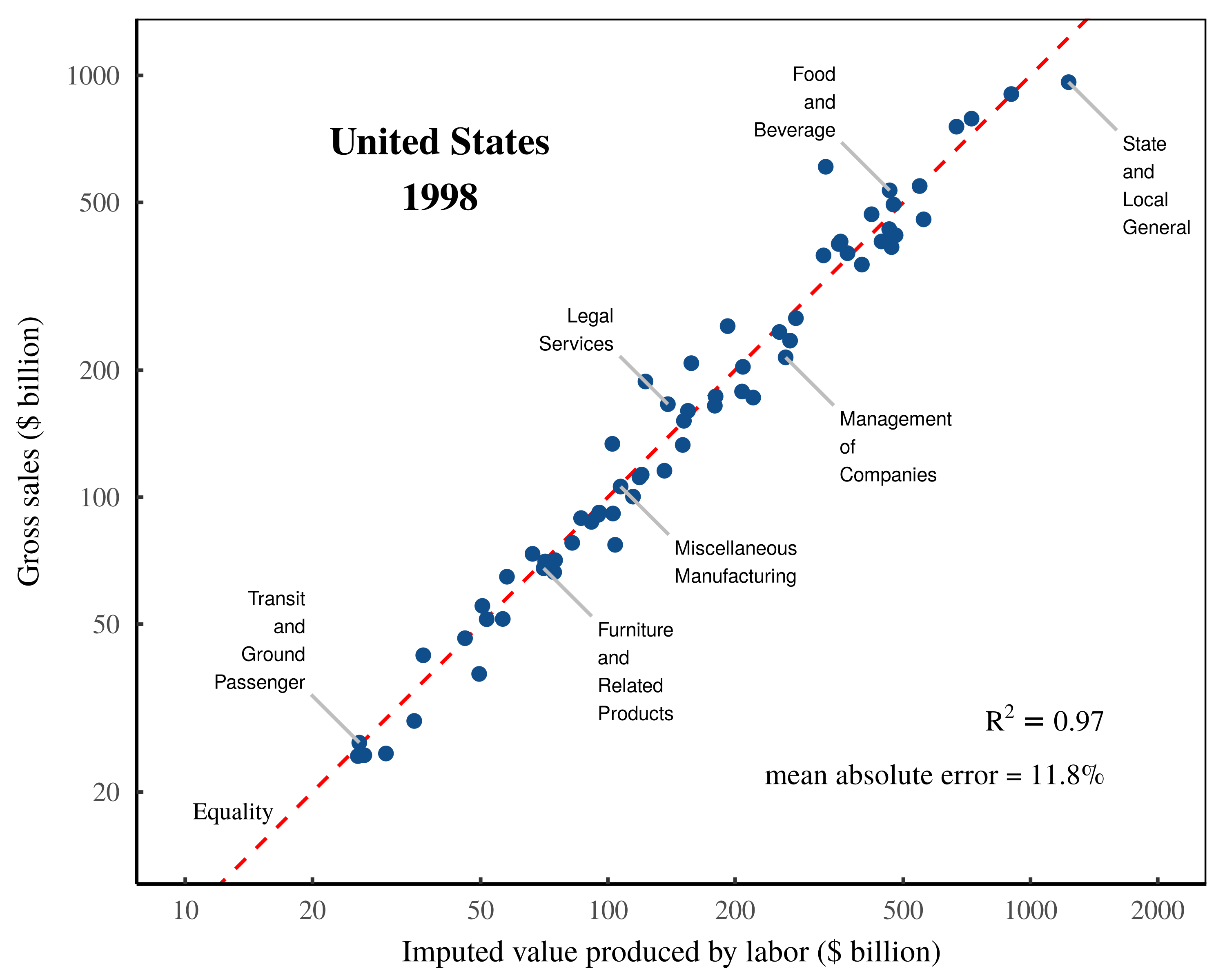Figure 1: Testing the labor theory of value — Shaikh’s published results.

This chart shows Shaikh’s method for testing the labor theory of value. The horizontal axis plots his data for the total imputed labor value embodied in each sector’s ‘gross output’. The vertical axis plots the corresponding monetary value of this ‘output’, as measured by gross sales. Note that both axes use a log scale. The data is from Appendix 9.3 of Shaikh’s online repository. The $\footnotesize R^2$ value is calculated on a log-log regression. The dashed-red indicates a one-to-one relation between labor values and gross sales. The mean error is calculated as the mean absolute difference between sectoral gross sales and imputed labor values, expressed as a percentage of sectoral gross sales.

Before unpacking the circularity in Shaikh’s method, I will first demonstrate that I can reproduce his results. Figures 2 to 4 show my replication of Shaikh’s work, using US national accounts data downloaded in 2023.

The main hurdle to replicating Shaikh’s work turns out to be the national accounts data itself, which has changed since the time of Shaikh’s analysis. The US Bureau of Economic Analysis continuously updates its data with revised numbers and (in this case) revised sectoral categories. To directly replicate Shaikh’s published work, we must first recategorize the modern data to make it consistent with the sectors used by Shaikh. I have documented the steps for this transformation in the Appendix.

Likely because the underlying national accounts data has changed, my replication of Shaikh’s numbers has a small degree of error. Figure 2 shows my replication of sectoral gross sales. Figure 3 shows my replication of Shaikh’s imputed labor values. Despite the slight discrepancy in results, I am able to reproduce the extremely tight relation between imputed labor values and gross sales, illustrated in Figure 4.

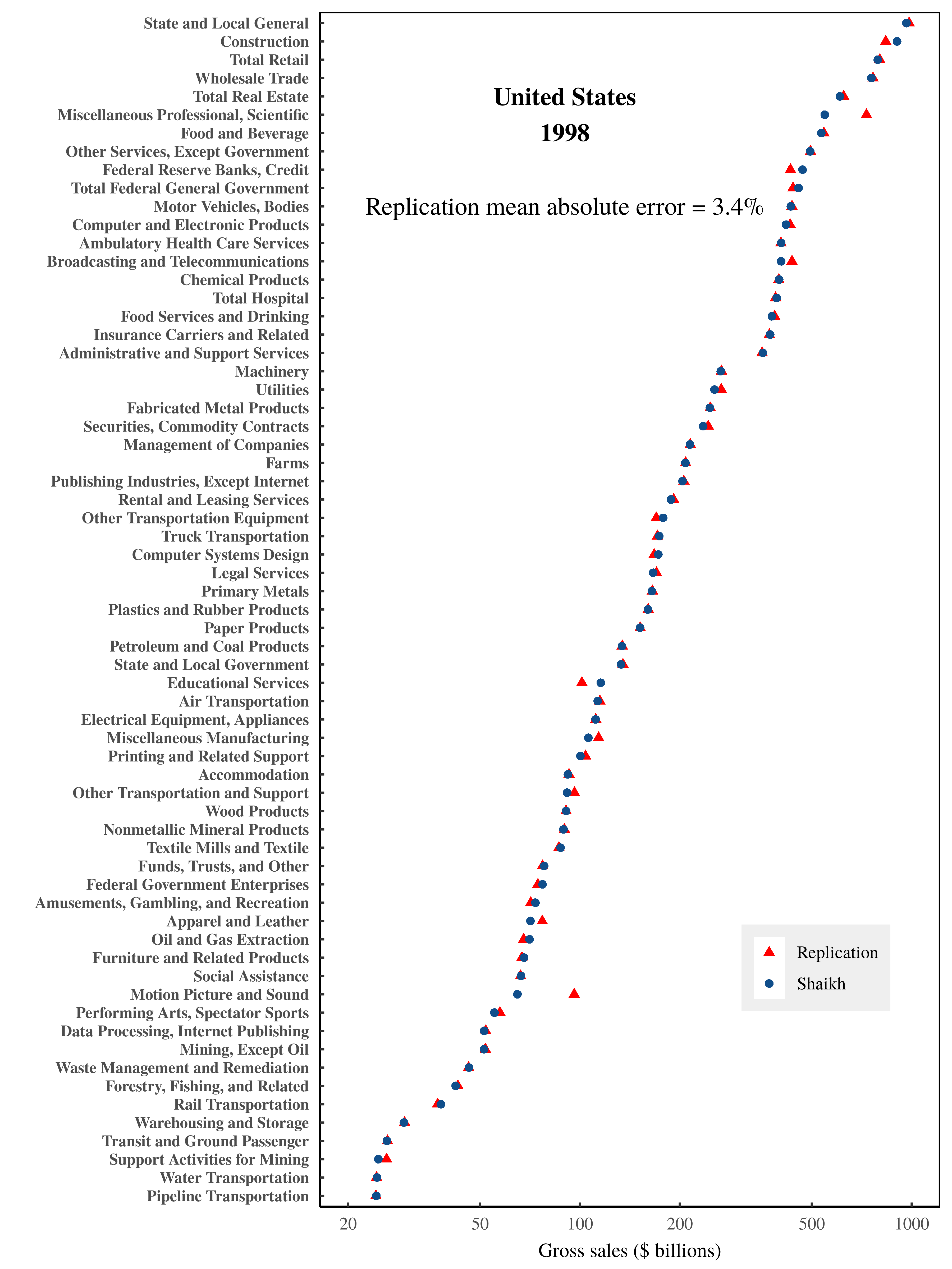Figure 2: Gross sales by US sector in 1998 — a replication of Shaikh’s data.

Blue points show Shaikh’s published values for US sectoral gross sales in 1998, taken from Appendix 9.3 of his online repository. (Shaikh refers to this data as ‘market prices’.) Red triangles show my replicated data, which has a mean error of roughly 3%. Note that the horizontal axis uses a log scale. For the data and methods behind this analysis, see the Appendix.

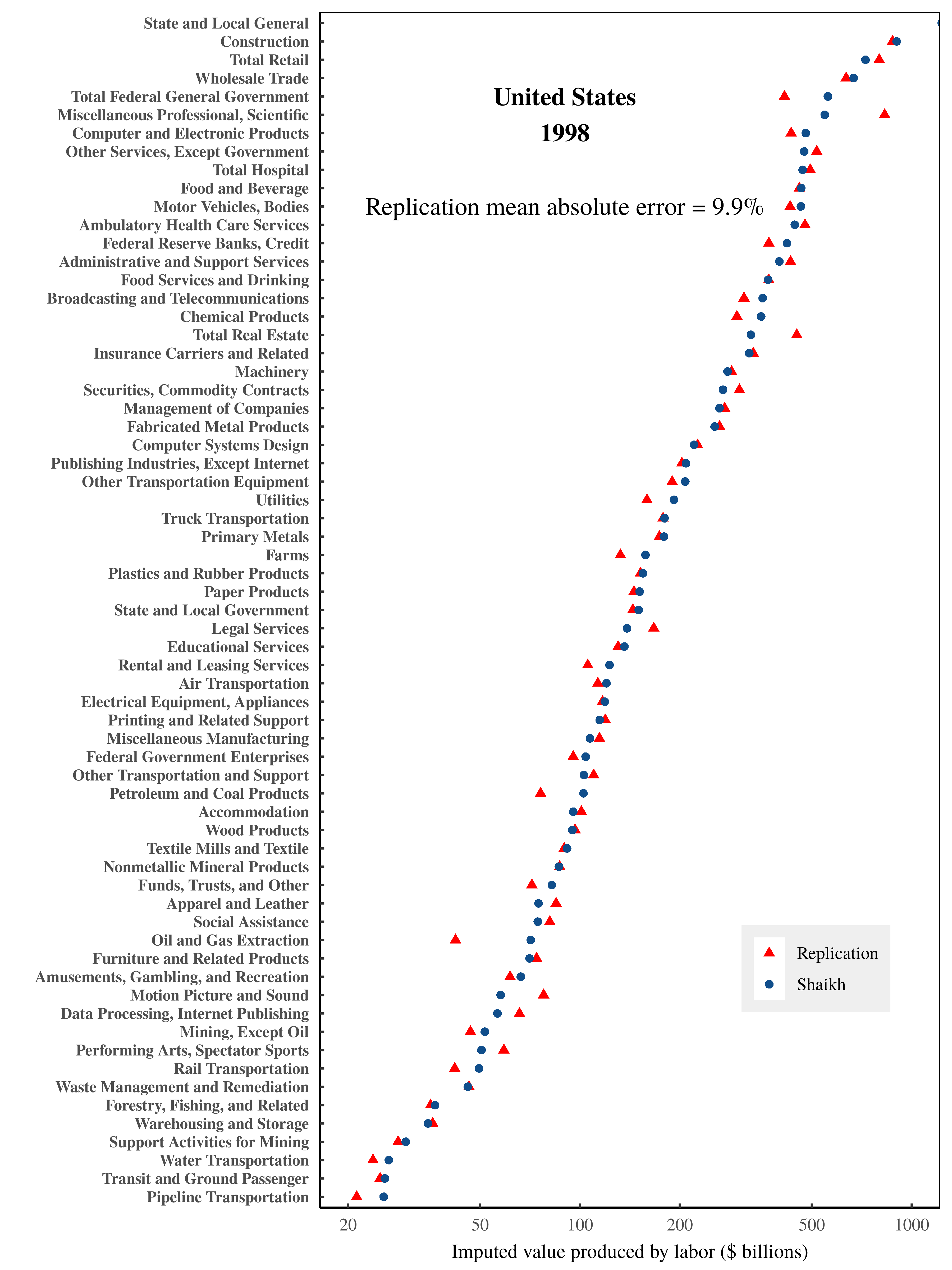Figure 3: Imputed labor value by US sector in 1998 — a replication of Shaikh’s results.

Blue points show Shaikh’s published values for imputed labor values by US sector in 1998. (Shaikh refers to this data as ‘direct prices’). Data is from from Appendix 9.3 of his online repository. Red triangles show my replicated data, which has a mean error of roughly 10%. Note that the horizontal axis uses a log scale. For the data and methods behind this analysis, see the Appendix.

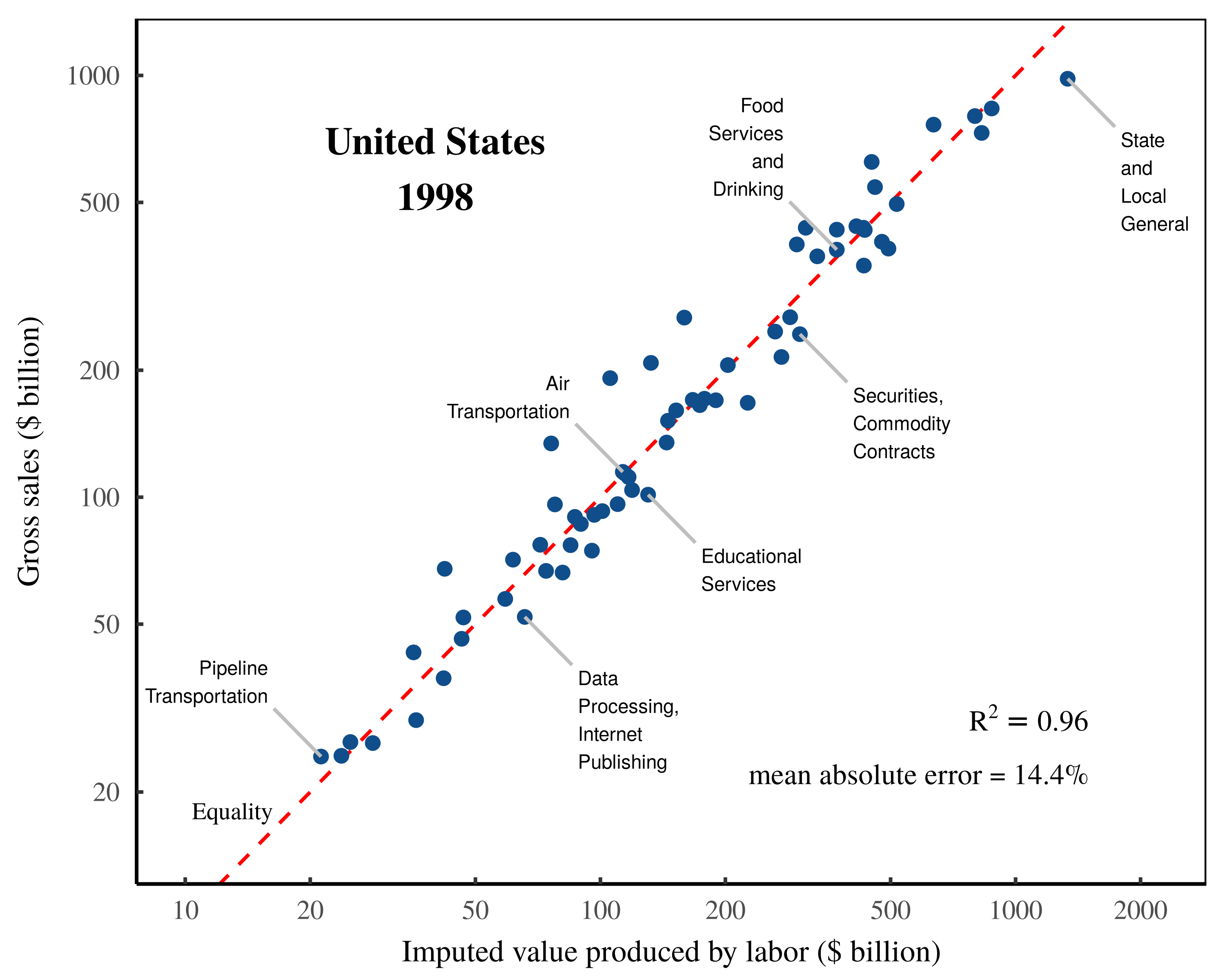Figure 4: Gross sales vs. imputed labor values — a replication of Shaikh’s analysis.

This chart shows my replication of Shaikh’s method for testing the labor theory of value. The horizontal axis plots total imputed labor values within each sector. The vertical axis plots each sector’s gross sales. Note the log scale on both axes. The $\footnotesize R^2$ value is calculated on a log-log regression. The mean error is calculated as the mean absolute difference between sectoral gross sales and imputed labor values, expressed as a percentage of sectoral gross sales. The dashed-red indicates a one-to-one relation between imputed labor values and gross sales. For the data and methods behind this analysis, see the Appendix.

Does the empirical data actually matter?

Having replicated Shaikh’s results, let us now turn to the underlying circularity in his methods. Because Shaikh uses detailed national accounts data to impute labor values, one would assume that this data actually matters for generating the observed results. In what follows, I will demonstrate that the opposite appears true. Because Shaikh’s method appeals to underlying accounting identities, it turns out that we can fill the input data with nonsense and still recover a tight relation between imputed labor values and gross sales.

To outline the road ahead, I introduce three random datasets that I then input (consecutively) into Shaikh’s method. Each dataset progressively ramps up the nonsensicalness of the underlying economic relations. The silliness culminates in a ‘use table’ inscribed with the word ‘HUMBUG’. Despite the absurdity of the inputted data, in each case, I find that Shaikh’s method returns an apparent verification of the labor theory of value.

The real world, scrambled

My first nonsense dataset consists of real-world US sectoral data that has been randomly scrambled among sectors. The details of this ‘Scrambled Dataset’ are described in the Appendix. But at a high level, I construct this dataset by taking real-world data for sectoral gross sales, value added, and labor compensation and then randomly reassigning the elements of each ‘vector’ to a new sector.² (Each of the three vectors are independently permuted.) Then I backfill the relevant input-output tables with data that is random, but which still satisfies the required national accounting identities. The resulting dataset has sectoral data that is realistically distributed at surface level, but which has bizarre internal dynamics.

For example, in this scrambled dataset, the ‘Motion Picture and Sound Recording’ sector spends most of its money purchasing ‘Waste Management’ services. Likewise, the ‘Utilities’ sector spends almost nothing on ‘Petroleum and Coal’, but spends a fortune on ‘Furniture’. Similarly absurdities are found across the board (including in the ‘make table’, where we find that most industries sell a mix of commodities from outside their sector). Employment compensation is also bizarre. Workers in ‘Amusements, Gambling, and Recreation’ earn an average annual salary of $1.4 million. Meanwhile Federal government workers earn a paltry $3,000 per year.

Given this silliness, one might think that inputting this scrambled data into Shaikh’s method would ruin the tight relation between gross sales and imputed labor values. However, that is not what happens. Instead, the scrambled data also returns a tight relation, as illustrated in Figure 5. It would seem, then, that the real-world relations between sectors are somehow irrelevant to Shaikh’s test of the labor theory of value. Oddly, scrambled data performs just as well.

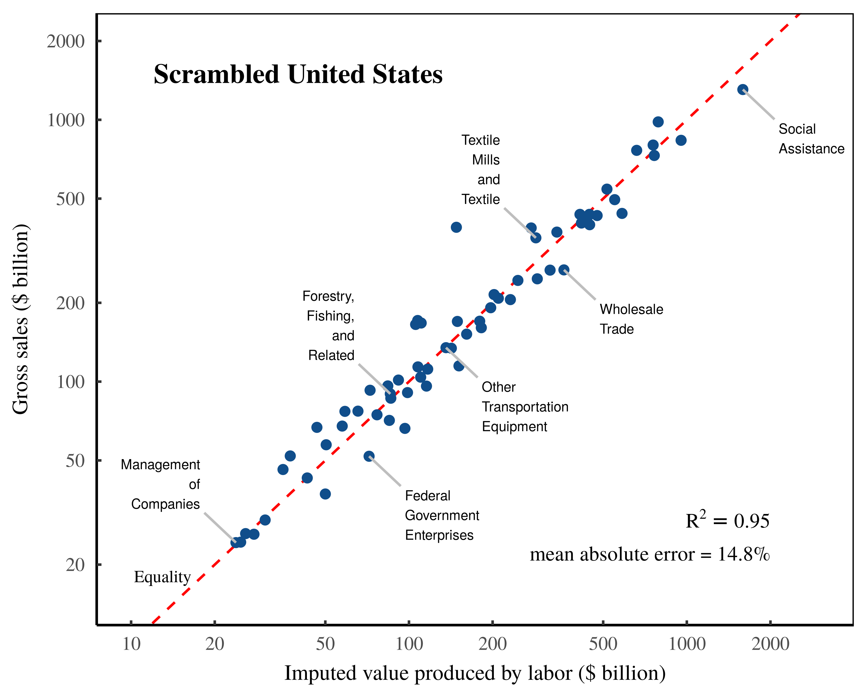Figure 5: ‘Validating’ the labor theory of value on scrambled US data.

This chart illustrates my replication of Shaikh’s method, applied to US data that has been scrambled into nonsense. To generate the scrambled data, I take real-world values for each sector’s gross sales, value added, and employment compensation, and then randomly reassign each element to a new sector. Then I backfill the input-output tables with random data that nonetheless satisfies the required national accounting identities. Finally, I input this scrambled data into Shaikh’s method for imputing labor values. Despite the scrambled nature of the underlying data, the results still appear to vindicate the labor theory of value. The $\footnotesize R^2$ value is calculated on a log-log regression. The mean error is calculated as the mean absolute difference between sectoral gross sales and imputed labor values, expressed as a percentage of sectoral gross sales. The dashed-red indicates a one-to-one relation between imputed labor values and gross sales. For the detailed methods behind this analysis, see the Appendix.

A random world

Continuing to explore how Shaikh’s method performs with randomized data, I now introduce what I call the ‘Random Numbers’ dataset. In this dataset, every input is a random number, pulled arbitrarily from a statistical distribution. (See the Appendix for details.) As such, this dataset is best regarded as statistical noise — but of a particular kind. Because the underlying data must respect national accounting identities, the various elements are both random yet bound to be interrelated.

(Note: For an extra dose of non-realness, the ‘Random Numbers’ data sets wages to be a tiny fraction of total income, meaning it is difficult to understand how the labor theory of value could apply to this data.)

Despite this data being meaningless noise, when we input it into Shaikh’s method, we again find a tight relation between gross sales and imputed labor values. Figure 6 shows the results. To summarize, it seems like Shaikh’s method is remarkably insensitive to the data it is given. Even when fed random noise, it still appears to ‘verify’ the labor theory of value.

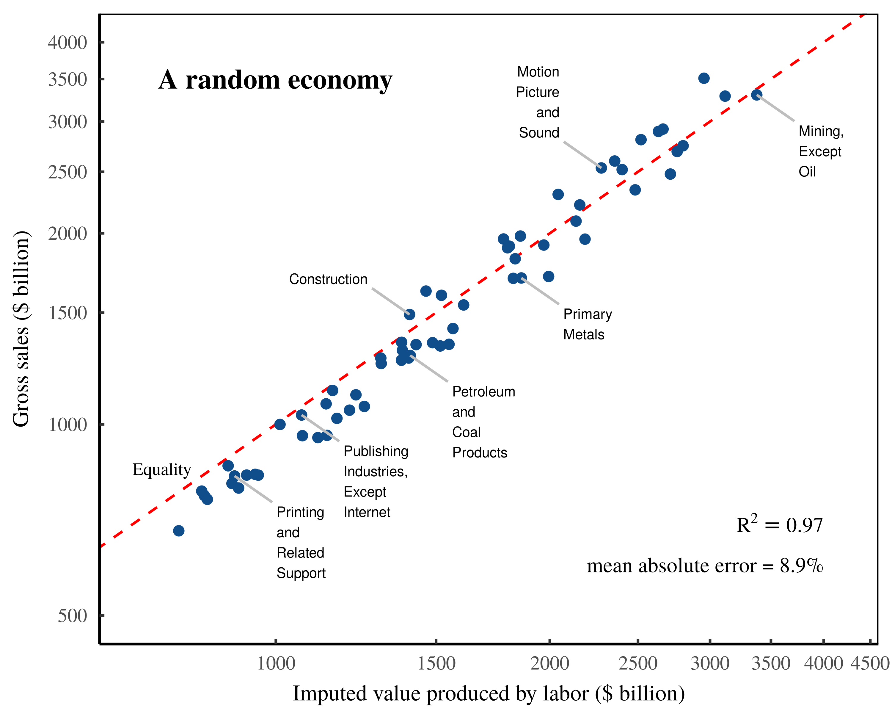Figure 6: ‘Validating’ the labor theory of value with random noise.

This chart illustrates my replication of Shaikh’s method, applied to completely random data. This data is generated by filling the ‘use table’ with random values from a lognormal distribution. The remaining data is then backfilled such that it meets the required national accounting identities. Despite the completely random nature of this data, the results still appear to vindicate the labor theory of value. The $\footnotesize R^2$ value is calculated on a log-log regression. The mean error is calculated as the mean absolute difference between sectoral gross sales and imputed labor values, expressed as a percentage of sectoral gross sales. The dashed-red indicates a one-to-one relation between imputed labor values and gross sales. For the detailed methods behind this analysis, see the Appendix.

A HUMBUG economy

To up the ante on meaningless data input, I will now take a cue from Shaikh himself. In his seminal 1974 paper, Shaikh demonstrated that one could use the Cobb-Douglas production function to ‘fit’ input data that spelled the word ‘HUMBUG’. The reason this bizarre operation worked, Shaikh showed, was because the Cobb-Douglas function was (under real-world conditions) a restatement of national accounting identities.

Intriguingly, the same principle appears to hold for Shaikh’s own method for testing the labor theory of value. We can input into this method nonsense data which spells ‘HUMBUG’, but nonetheless recover an apparent verification of the labor theory of value.

To demonstrate this principle, I begin with real-world US data from the 1998 ‘Commodity-by-Industry Use Table’. (For details about how this table enters into Shaikh’s method, see the Appendix.) Onto this real-world data, I then write the word ‘HUMBUG’ across the table by filling the relevant cells with the number ‘11111111111’. Figure 7 shows a screenshot of the resulting spreadsheet.

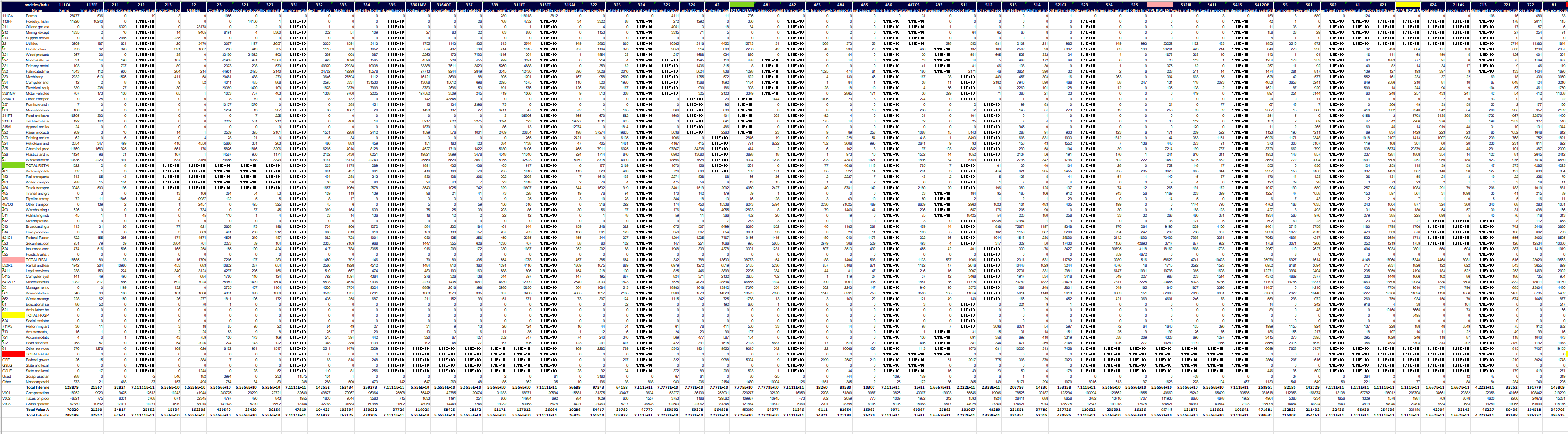Figure 7: The HUMBUG use table.

The ‘HUMBUG’ use table begins with data from the real-world 1998 US use table (downloaded from the Bureau of Economic Analysis). Across this table, I then write the word ‘HUMBUG’ using cells filled with ones.

With this ‘HUMBUG’ use table, I then use national accounting identities to define and fill the remaining quantities required by Shaikh’s method. (Again, for details, see the Appendix.) Finally, I input the ‘HUMBUG’ dataset into Shaikh’s equations, and calculate the implied labor values. Despite the absurdity of the underlying data, Shaikh’s method again returns an apparent verification of the labor theory of value.

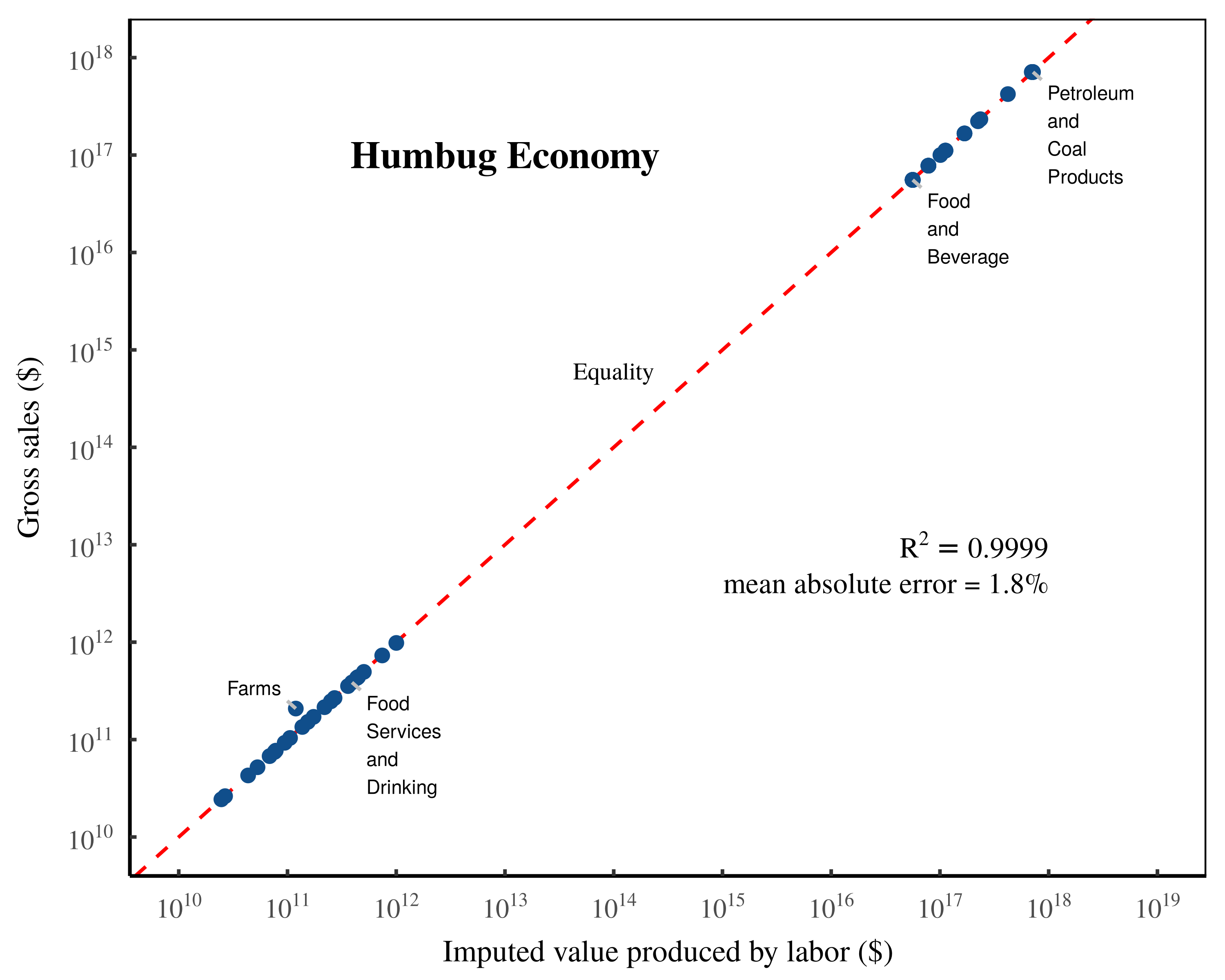Figure 8: ‘Validating’ the labor theory of value with HUMBUG data.

This chart shows my replication of Shaikh’s method based on a ‘use table’ that spells ‘HUMBUG’ across the spreadsheet with cells filled with ones. The resulting data is obviously absurd. (Sectors impacted by the ‘HUMBUG’ letters get a million-fold bump to their gross sales, and have intermediate expenses that are bizarre.) Still, Shaikh’s method reports back a tight fit between sectoral gross sales and imputed labor values. The $\footnotesize R^2$ value is calculated on a log-log regression. The mean error is calculated as the mean absolute difference between sectoral gross sales and imputed labor values, expressed as a percentage of sectoral gross sales. The dashed-red indicates a one-to-one relation between imputed labor values and gross sales. For the detailed methods behind this analysis, see the Appendix.

Testing an accounting identity

What we learn from the preceding exercise is that Shaikh’s method is strikingly insensitive to the data it is fed. Much like the Cobb-Douglas production function, Shaikh’s ‘test’ of the labor theory of value seems to readily accommodate data that is nonsense, nonetheless returning a tight correlation between imputed labor values and gross sales.

The reason for this apparent contradiction is that, like the Cobb-Douglas production function, Shaikh’s method for ‘testing’ the labor theory of value amounts to a ‘test’ of national accounting identities. Under the hood, Shaikh’s imputed labor values are actually a function of the quantity they seek to explain. As such, the method appears to ‘work’ irrespective of the data it is fed.

In the Appendix, I detail the exact steps behind this circularity. But here, I will note that the circularity is evident from the very start. Shaikh’s method for testing the labor theory of value is derived from Marx’s ‘fundamental equation of price’, a formula that decomposes a commodity’s price into three components:

$\displaystyle p = ulc + m + a\qquad{(4)}$

Here, $\footnotesize ulc$ represents unit labor costs, $\footnotesize m$ is unit profits, and $\footnotesize a$ is unit intermediate expenses. The problem with this starting point is that it contains nothing to test. Marx’s equation is not a falsifiable ‘hypothesis’; it is an accounting identity that is defined to be true by the rules of double-entry bookkeeping. As such, when we manipulate this equation, we are simply manipulating a pre-defined identity.

Shaikh’s contribution is to take Marx’s accounting identity and transform it using Sraffa’s methods for input-output decomposition. The goal is to decompose the intermediate expense term $\footnotesize a$ into a series of labor cost and profit terms that are paid out through an ever expanding web of transactions. That is, since $\footnotesize a$ is itself a price, it can be expressed recursively as the sum of labor costs, profit, and intermediate expenses spent on another commodity:

$\displaystyle a = ulc_1 + m_1 + a_1 \qquad{(5)}$

If we follow this recursion to its logical conclusion, we can express a commodity’s price in terms of a series of labor expenses and profit terms:

$\displaystyle \begin{aligned} p &= ulc + m + a \\ &= ulc + m + ulc_1 + m_1 + a_1 \\ &= ulc + m + ulc_1 + m_1 + ulc_2 + m_2 + a_2 + \ldots \\ & = ulc + ulc_1 + ulc_2 + ulc_3 + \ldots + m + m_1 + m_2 + m_3 + \ldots \end{aligned} \qquad{(6)}$

The result of this decomposition is that Shaikh is able to rewrite Marx’s identity in terms of two forms of income. The series of $\footnotesize ulc$ terms sum to what Shaikh calls ‘vertically integrated unit labor costs’, $\footnotesize vulc$ . And the series of profit terms $\footnotesize m$ sum to what Shaikh calls ‘vertically integrated unit profits’, $\footnotesize vm$ .

$\displaystyle p = vulc +vm \qquad{(7)}$

Tellingly, Shaikh notes that this price equation can be rewritten as follows:

$\displaystyle p = vulc \cdot ( 1 + \sigma_{pw} ) \qquad{(8)}$

Here, $\footnotesize \sigma_{pw}$ is the ratio of vertically integrated unit profits to vertically integrated unit wages:

$\displaystyle \sigma_{pw} = \frac{vm}{vulc}\qquad{(9)}$

Since Eq. 8 is simply a rearrangement of Marx’s accounting identity, it still contains nothing to test. But Shaikh’s method looks at this identity and presumes that there is something to test. That is, Shaikh’s method looks at vertically integrated labor costs and sees the Marxist concept of ‘labor value’. It then correlates these labor costs (‘values’) back to prices, forgetting that this correlation is an exercise in double-entry bookkeeping.

Indeed, the accounting identity in Eq. 8 spells out the conditions required for Shaikh’s ‘test’ to succeed. To find a high correlation between prices and vertically integrated labor costs, the noise term $\footnotesize \sigma_{pw}$ must get out of the way, either by being negligibly small, or by not varying much across commodities.

Looking at this noise term, we see that it is the ratio of vertically integrated profits to vertically integrated wages. In short, if this ratio is small — meaning profits are dwarfed by wages — Shaikh’s method is guaranteed to return a high correlation between prices and vertically integrated labor costs. Likewise, if the ratio of profits to wages is fairly consistent across commodities, the noise term reduces to a constant, thereby guaranteeing a tight correlation between prices and vertically integrated labor costs.

When Shaikh re-implements Marx’s identity to fit with the sectoral data in the national accounts, the same principle holds. If income shares are relatively stable across sectors, the underlying accounting identity guarantees a tight relation between Shaikh’s imputed labor values and sectoral gross sales.

It is for this reason that Shaikh’s method seems to accommodate nonsense data. For the most part, the inputted national accounts data serves mostly as a pawn to be manipulated by accounting identities. The data that actually seems to matter is the income composition across sectors.

To demonstrate this fact, Figure 9 takes the four datasets studied here — the ‘Replication dataset’, the ‘Scrambled dataset’, the ‘Random Numbers dataset’ and the ‘HUMBUG dataset’ — and calculates the cross-sector dispersion in the labor share of income. As this dispersion increases, the tightness of the results (measured by the $\footnotesize R^2$ value between gross sales and imputed labor values) tends to decrease.³

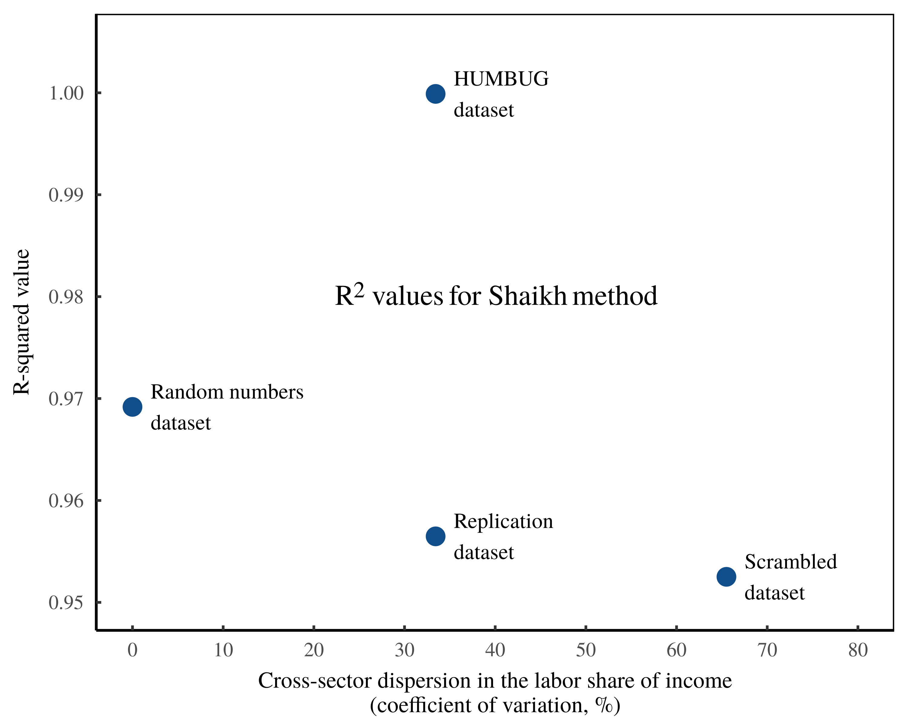Figure 9: The tightness of the Shaikh method seems to be tied to cross-sector variation in the labor share of income.

In this chart, each point represents one of the datasets studied here (the Shaikh replication dataset, the ‘scrambled’ dataset, the ‘random’ dataset, and the ‘HUMBUG’ dataset). The vertical axis shows, for each dataset, the $\footnotesize R^2$ value for a log-log regression between sector gross sales and imputed labor values. The horizontal axis plots, for each dataset, the cross-sector dispersion in the labor share of income (measured using the coefficient of variation). The ‘HUMBUG’ data not withstanding, the tightness of the Shaikh method appears to decrease as cross-sector labor income becomes more dispersed.

To summarize, Shaikh’s method appears to ‘verify’ the labor theory of value for the same reason that the Cobb-Douglas production function appears to ‘verify’ neoclassical theories of economic growth. Both approaches amount to restatements of national accounting identities. And both approaches become circular when the labor share of income remains roughly constant.

Economics is not physics

Shaikh’s work amounts to an elegant interpretation of Marxist theory, restated though the lens of Sraffian analysis. Its elegance, however, cannot overcome the core flaw in the labor theory of value, which is that Marxist labor values are fundamentally unobservable.

For Marx, ‘labor value’ consists of an infinitely fungible universal quantum that represents the social relation of an average socially necessary abstract unit of labor. In order to objectively measure such a quantity, one needs to overcome a series of (unsurpassable) hurdles. First, one must take by-the-clock labor time and objectively adjust for the value-producing skill of different workers. Second, one must objectively differentiate between labor which is ‘socially necessary’, and that which is not. Third, one must adjust for a wide variety of real-world complications, including joint production, the production of byproducts, heterogeneous production processes, market power, economies of scale, coercion, and so on. Finally, if the resulting imputed labor values are to be useful for explaining prices, then the entire measurement process must be done without any reference to monetary value.

Perhaps recognizing the futility of this task, empirically minded Marxists make no attempt to estimate labor values independently from prices. Instead, they do the exact opposite: they infer labor value from prices — the very thing that the labor theory of value is supposed to explain. In their seminal book Capital as Power, Nitzan and Bichler break down this road to tautology:

Recall that, according to Marx, the value of a commodity denotes the abstract labour time socially necessary for its production. Yet […] this quantum is impossible to measure. And so the researcher makes assumptions.

The most important of these assumptions are that the value of labour power is proportionate to the actual wage rate, that the ratio of variable capital to surplus value is given by the price ratio of wages to profit, and occasionally also that the value of the depreciated constant capital is equal to a fraction of the capital’s money price. In other words, the researcher assumes precisely what the labour theory of value is supposed to demonstrate […]

In short, we have to pretend. Since values are forever unknown, we need to first convert prices into ‘values’ and then correlate the result with prices. It seems reasonable to expect the outcome to be positive and tight. After all, we are correlating prices with themselves. What remains unclear is why one would bother to show this correlation, and more puzzling still, how the whole exercise relates to the labour theory of value.

(Nitzan & Bichler, 2009, p. 97)

Because Shaikh’s empirical work commits exactly this sin — using monetary data to impute labor values and then demonstrating that these values correlate tightly with monetary value — it amounts to a rubber stamp for the labor theory of value. Indeed, one can input statistical nonsense into Shaikh’s equations and still appear to ‘verify’ the labor theory of value.⁴

Intriguingly, it appears that the main condition for this operation to work is that income composition is relatively consistent across sectors. But this feature of the real world is entirely unsurprising — it is a natural consequence of capital and labor mobility, in which both capitalists and workers move sectors to chase higher profits and higher wages.

To be fair to Shaikh, the root of these problems lies with Marx himself. While Marx was a savvy social critic who was well aware of the complexities of real-world capitalism, he was also impressed by the success of the emerging natural sciences. As such, Marx’s attempt at a ‘scientific’ theory of capitalism ended up naively assuming that ‘value’ was governed by deterministic equations. But in the end, the only way that real-world complexities could be suitably flattened was for the theory to assume what it aimed to prove. Thus we have the enduring contradiction that labor values simultaneously explain and are revealed by prices.

Unfortunately, Marx’s appeal to natural-science-like determinism is a mistake that continues to be made by many contemporary economists, be they Marxist, neoclassical, Keynesian, or otherwise. The problem is ultimately that economics cannot be reduced to social physics. It is, however, socially expedient for economists to pretend the opposite. Indeed, the cloak of deterministic mathematics is a powerful way to obscure the circularity of a theory, just as the cloak of Latin was a powerful way for the Catholic Church to obscure the flaws in its theosophical apologia. Now as then, (secular) priests use linguistic arcaneness to mask basic logical mistakes.

As a rule, if a researcher attempts to reduce the complexities of the human experience (including the gyrations of whole societies) to a mechanical equation, it is a sign that something has gone terribly wrong. True, under certain limited circumstances, aggregate human behavior can sometimes be numerically predictable. For example, at a grocery store, impulse purchases such as candy may sell 7% more when placed next to the cash register instead of at the back of the store. However, this predictability must be treated with scientific humility because it rarely extends to socio-economic systems as a whole. When it comes to large-scale human behavior, deterministic models typically fall short because they exclude the phenomenon of qualitative novelty. Nicholas Georgescu-Roegen explains:

The most important aspect of the economic process is precisely the continuous emergence of novelty. Now, novelty is unpredictable, but in a sense quite different from the way in which the result of a coin toss is unpredictable… [it] is unique in the sense that in chronological time it occurs only once. Moreover, the novelty always represents a qualitative change. It is therefore understandable that no analytical model can deal with the emergence of novelty, for everything that can be derived from such a model can only concern quantitative variations. Besides, nothing can be derived from an analytical model that is not logically contained in its axiomatic basis.

(Georgescu-Roegen, 1979, quoted in Nitzan and Bichler, 2009, p. 325)

The failure to incorporate qualitative novelty is precisely the problem with the labor theory of value, which purports to explain the novel dynamics of a complex social system in terms of an almost comically deterministic formula. But despite what Marx sometimes claimed, the future is qualitatively uncertain.

For example, what forward-looking capitalist, buying timberland in the early 1700s, could price into his capitalization model the decreasing value of timberland caused by the invention of steam engines, which by pumping water out of coal mines, would soon make coal cheaper than wood? Likewise, what 1980s music industry mogul could have predicted the rise of online music streaming, much less the internet, 30 years later?

The answer is obviously that no one could have predicted these novel changes. And yet despite this inability to predict a fundamentally novel future, capitalists are still tasked with doing so in pricing their assets (and by extension, their commodities) based on expected future income streams. Given this innate uncertainty, commodity and asset pricing is not an effort in objective accounting; it is a collective guessing-game.

For this reason, mechanistic theories of value will always fail. And if such theories do appear to succeed, it is generally because their premises are circular. After all, assuming what one aims to prove is a reliable method for generating a tautological theory that is definitionally infallible.

On this front, the labor theory of value is by definition untestable, since labor values cannot be observed without inferring them from prices. And once we use prices to infer labor values, we leave behind the world of predictive science and enter the rule-bound domain of double-entry bookkeeping — a world in which correlations readily spring forth from underlying accounting identities.

It is in this world of accounting identities that Anwar Shaikh made his most enduring contribution to political economy. In his seminal 1974 paper, Shaikh demonstrated that a generation of neoclassical economists had been mislead by the empirical ‘success’ of the Cobb-Douglas function. The equation worked, Shaikh demonstrated, not because it uncovered some fundamental truth about capitalist production, but because under real-world conditions, it was a restatement of national accounting identities.

The irony is that Shaikh’s own work appears to fall victim to the same problem. When ‘testing’ the labor theory of value, Shaikh is actually rearranging national accounting identities in such a way that the ‘test’ is almost guaranteed to succeed, regardless of the data it is fed. Indeed, the double irony is that the conditions for this ‘success’ seem to be a slight variation on the conditions that Shaikh identified in his deconstruction of the Cobb-Douglas equation. If the labor share of income is fairly consistent across sectors, Shaikh’s method will deliver a tight relation between imputed labor values and sectoral gross sales, even when using nonsense data that spells ‘HUMBUG’. In short, the apparent ‘empirical strength’ of the labor theory of value rests largely on the circular derivation of labor values — a derivation that appeals not to the laws of capitalism, but to the laws of double-entry bookkeeping.

Appendix

Links to data

A zipped folder containing all the data and materials used in this paper is available at the Open Science Framework: https://osf.io/5za2c

Note that the notation used in the spreadsheets corresponds to Shaikh’s notation in his essay The Transformation from Marx to Sraffa, Appendix B, which is more comprehensive than his explanation in Capitalism: Competition, Conflict, Crises.

Table 1: A glossary of terms used in Shaikh’s method

$\footnotesize (\boldsymbol{I}-\boldsymbol{A}^{\prime})^{-1}$	The US Industry-by-Industry Total Requirements Table, reported by the Bureau of Economic Analysis (BEA). In national accounting jargon, the total requirements table measures the sum of total direct and indirct inputs from industry $\footnotesize i$ per unit of output in industry $\footnotesize j$ . Jargon aside, this table is a bookkeeping matrix that tracks the sum of direct and indirect expenses paid to sector $\footnotesize i$ per dollar of sales in sector $\footnotesize j$ .
$\footnotesize \boldsymbol{A}$	A hypothetical input-output matrix inspired by Sraffian analysis. Each element, $\footnotesize x_i / x_j$ , consists of the quantity of commodity $\footnotesize i$ directly used to produce one unit of commodity $\footnotesize j$ . This matrix cannot be derived from national accounts data.
$\footnotesize \boldsymbol{A}^{-1}$	Denotes the inverse of matrix $\footnotesize \boldsymbol{A}$ .
$\footnotesize \boldsymbol{A}^{\prime}$	The Industry-by-Industry Direct Requirements Table. In national accounting jargon, this matrix tracks the direct inputs from sector $\footnotesize i$ used per unit of output in sector $\footnotesize j$ . Jargon aside, the direct requirements table is a bookkeeping matrix that tracks the direct expenses paid to sector $\footnotesize i$ per unit of sales in sector $\footnotesize j$ .
$\footnotesize \boldsymbol{c}$	A vector of labor compensation measured across all sectors.
$\footnotesize c_j$	Labor compensation in sector $\footnotesize j$ .
commodity view	A method for categorizing sectors that (to some degree) dissects firm boundaries and categorizes transactions based on their perceived form. In national accounting jargon, the commodity view is called ‘commodity use’ and ‘commodity output’.
direct prices	Shaikh’s (misleading) term for the normalized imputed labor values measured across all US sectors. $\footnotesize \text{direct prices} = \boldsymbol{v}^{\prime} \cdot \mu$
$\footnotesize e_j$	The employment in sector $\footnotesize j$ .
$\footnotesize \boldsymbol{f}$	A vector of value added measured across all sectors, where transactions are classified according to the ‘commodity view’. (In national accounting jargon, $\footnotesize \boldsymbol{f}$ is called ‘final commodity demand’.)
$\footnotesize \boldsymbol{g}$	A vector of gross sales measured across all sectors, where transactions are categorized according to the ‘industry view’. (In national accounting jargon, gross sales are typically called ‘gross output’.)
$\footnotesize g_j$	The gross sales in sector $\footnotesize j$ , where transactions are categorized according to the ‘industry view’. (In national accounting jargon, gross sales are typically called ‘gross output’.)
$\footnotesize \boldsymbol{I}$	An identity matrix. $\footnotesize \boldsymbol{I}$ consists of a square matrix that contains only ones on its diagonal, and zeros for all other values.
$\footnotesize \boldsymbol{i}$	A column vector containing only ones. In linear algebra, this vector is used to calculate the row sums or the column sums of a matrix.
industry view	A method for categorizing sectors based on firm boundaries. Firms are placed within a sector based on their primary source of revenue. In national accounting jargon, the ‘industry view’ of each sector is refered to as an ‘industry’.
$\footnotesize \boldsymbol{l}$	A vector of per-unit direct labor values measured across all commodities. This vector cannot be derived from national accounts data.
$\footnotesize \boldsymbol{l}^{\prime}$	A vector of labor value per dollar of gross sales measured across all sectors.
$\footnotesize \iota_j$	A measure of direct labor value in sector $\footnotesize j$ . According to Marxist theory, this measurement should be denoted in units of socially necessary abstract labor time. But since such units are unobservable, empirically minded Marxists typically turn to measures of labor income to proxy ‘labor value’.
$\footnotesize l^{\prime}_j$	The direct labor value per dollar of gross sales in sector $\footnotesize j$ .
$\footnotesize l_j$	The direct labor value per unit of commodity $\footnotesize j$ . This hypothetical quantity cannot be derived from national accounts data.
market prices	Shaikh’s (misleading) term for sector gross sales, $\footnotesize \boldsymbol{g}$ .
$\footnotesize \mu$	In Marxist jargon, $\footnotesize \mu$ is the “monetary expression of labor time” — the number of currency units which denote one unit of socially necessary abstract labor time. In Shaikh’s method, $\footnotesize \mu$ is a normalization constant designed such that the sum of the direct price vector is equivalent to the sum of the gross sales vector $\footnotesize \boldsymbol{g}$ .
$\footnotesize p_j$	The price of commodity $\footnotesize j$ . The goal of the labor theory of value is to explain this price. However, the lack of commodity-level data makes this goal essentially untestable.
$\footnotesize \boldsymbol{q}$	The vector of gross sales measured across all sectors, classified according to the ‘commodity view’. (In national accounting jargon, $\footnotesize \boldsymbol{q}$ is called ‘gross commodity output’.)
$\footnotesize \boldsymbol{U}$	The BEA Commodity-by-Industry Use Table. In national accounting jargon, the ‘use table’ quantitifies the ‘use of commodities’ by each respective ‘industry’. Jargon aside, the ‘use table’ is a bookkeeping matrix that measures expense transactions across sectors. On the purchasing end, sectors are classified according to the ‘industry view’, in which firms are placed into sectors based on their primary source of revenue. On the receiving end, sectors are classified according to the ‘commodity view’, meaning firm boundaries are (to some degree) ignored and each transaction is placed into a sector based on its perceived type.
$\footnotesize \boldsymbol{V}$	The BEA Industry-by-Commodity Make Table. In national accounting jargon, the ‘make table’ measures ‘commodity output’ by ‘industry’. Jargon aside, the ‘make table’ is a bookkeeping matrix, which presents two views for sectoral gross sales. In the industry view, sales are lumped into sectors based on each firm’s primary source of revenue. In the make table, these sales are then decomposed into a corresponding ‘commodity view’, in which firm boundaries are ignored, and transactions are lumped into sectors based on their perceived type. If all firms perfectly respected sectoral boundaries, the ‘make table’ would collapse to $\footnotesize \boldsymbol{ \widehat{g} }$ , a matrix with the gross sales vector along the diagonal, and all other elements equal to zero.
$\footnotesize \boldsymbol{v}$	A vector of per-unit labor values measured across all commodities. This vector cannot be derived from national accounts data.
$\footnotesize \boldsymbol{v}^{\prime}$	A vector of total labor values per dollar of gross sales measured across all sectors.
$\footnotesize v^{\prime}_j$	The total labor value per dollar of gross sales in sector $\footnotesize j$ .
$\footnotesize v_j$	The total per-unit labor value embodied in commodity $\footnotesize j$ . This quantity cannot be derived from national accounts data.
$\footnotesize \bar{w}$	The economy-wide average wage.
$\footnotesize \bar{w}_j$	The average wage in sector $\footnotesize j$ .
$\footnotesize x_j$	The output quantity of commodity $\footnotesize j$ , denominated in ‘natural units’ (as in ‘100 pencils’ or ‘500 apples’). This quantity cannot be derived from national accounts data.
$\footnotesize \boldsymbol{y}$	A vector of value added measured across all sectors. In the national accounts, ‘value added’ consists of gross sales less the intermediate expenses paid to other sectors.
$\footnotesize \widehat{~}$	When placed over a vector, the $\footnotesize \widehat{~}$ symbol represents taking the values of the vector and placing them on the diagonal of a square matrix, with all non-diagonal values set to zero.
$\footnotesize \circ$	Denotes element-wise multiplication of two vectors.
$\footnotesize \oslash$	Denotes element-wise division of two vectors.

Shaikh’s empirical method: Linear algebra and circular algebra

At a high level, Shaikh’s empirical method consists of a simple correlation; looking across US sectors, Shaikh compares each sector’s gross sales to the imputed value generated by labor. He finds a tight relation, which he interprets as a vindication of the labor theory of value. The problem, however, is that Shaikh’s imputation of labor values is circularly dependent on the monetary data he seeks to explain. In what follows, I will dissect the math. (See Table 1 for a glossary of terms.)

Imputing direct labor values

The centerpiece of Shaikh’s method is his imputation of ‘vertically integrated labor values’, a calculation that is designed to impute the total socially necessary abstract labor time embodied in each sector’s output. To reconstruct Shaikh’s reasoning, we will start with the simpler version of direct labor value, which restricts the method to the workers in each sector.

We begin with a hypothetical calculation. Suppose that sector $\footnotesize j$ produces the commodity $\footnotesize j$ with an output quantity $\footnotesize x$ . And suppose that in this sector, workers input $\footnotesize \iota$ hours of socially necessary abstract labor time. We can therefore state that in sector $\footnotesize j$ , the labor time per unit of output is:

$\displaystyle l_j = \frac{\iota_j} { x_j} \qquad{(10)}$

The purpose of this calculation is to mimic what should be explained by the labor theory of value. According to this theory, the price $\footnotesize p$ of commodity $\footnotesize j$ ought to be proportional to the socially necessary abstract labor time embodied in each commodity. As such, $\footnotesize p_j$ ought to correlate with per-unit labor direct labor time, $\footnotesize l_j$ :

$\displaystyle p_j \sim l_j \qquad{(11)}$

Of course, our comparison is so far incomplete, since we have not yet tracked the indirect labor time embodied in our commodity. We will amend this shortcoming later. First, however, we must deal with a more pressing problem, which is that the quantity of output, $\footnotesize x_j$ , is not directly observable.

The issue here is that our setup is somewhat misleading. Shaikh’s method has so far assumed that each sector produces a single commodity called $\footnotesize j$ . However, in the real world, there is no such commodity. That is because real-world sectors are large-scale aggregations of business activity, aggregations that sell thousands (if not millions) of different commodities. As such, we cannot speak about the ‘quantity of output’ without first introducing a dimension of aggregation.

For their part, economists typically chose price as their dimension of aggregation. The result is that economists infer ‘output’ by measuring aggregate monetary value. Of course this inference is allowable, but what it means is that the language of ‘output’ is a tacked-on assumption. What economists directly measure is gross sales — the aggregate gross revenue in each sector.

Following this standard economics procedure, Shaikh retains the language of ‘output’, but does not actually measure the output quantity $\footnotesize x_j$ . Instead, he infers ‘output’ by measuring each sector’s gross sales, $\footnotesize g_j$ . As such, Shaikh’s empirical measurement for ‘per-unit’ direct labor time relies on the following revised formula, which actually measures labor time per dollar of gross sales:

$\displaystyle l^{\prime}_j = \frac{ \iota_j}{ g_j } \qquad{(12)}$

Now to the task of measuring each sector’s (direct) socially necessary abstract labor time, $\footnotesize \iota$ . A good starting point is to equate labor time with the number of full-time equivalent workers employed in each sector, $\footnotesize e_j$ :

$\displaystyle \iota_j = e_j \qquad{(13)}$

Marxists would call sectoral employment, $\footnotesize e_j$ , by-the-clock labor time, since it counts the hours of all workers equally. In contrast, ‘socially necessary abstract labor time’ must account for the different value-creating ability of different workers. So how, then, do we measure this value-creating ability?

For his part, Shaikh uses workers’ wages as a proxy for their value-creating ability. As such he infers direct labor values by taking sectoral employment and multiplying it by his proxy for skill, the normalized average sectoral wage. His calculation of $\footnotesize \iota_j$ therefore becomes:

$\displaystyle \iota_j = \frac{ \bar{w}_j } { \bar{w} } \cdot e_j \qquad{(14)}$

Here $\footnotesize \bar{w}_j$ is the average compensation per employee in sector $\footnotesize j$ . And $\footnotesize \bar{w}$ is the average compensation per employee across the whole economy.

Let us now pause to think about what Shaikh is actually measuring. Although Eq. 14 carries the language of ‘labor time’, it is actually a measurement of monetary value. Here is the math. First, note that the sectoral average wage, $\footnotesize \bar{w}_j$ , is defined as a sector’s labor compensation, $\footnotesize c_j$ , divided by its employment, $\footnotesize e_j$ :

$\displaystyle \bar{w}_j = \frac{c_j}{e_j} \qquad{(15)}$

Substituting this formula back into Eq. 14 gives:

$\displaystyle \iota_j = \frac{ c_j / e_j } { \bar{w} } \cdot e_j \qquad{(16)}$

After cancelling the common $\footnotesize e_j$ terms, we find that our measurement of direct ‘labor time’ is purely financial; it takes a sector’s labor compensation, $\footnotesize c_j$ , and divides by the economy-wide average wage, $\footnotesize \bar{w}$ :

$\displaystyle \iota_j = \frac{ c_j } { \bar{w} } \qquad{(17)}$

Now let us return to Shaikh’s imputation of direct labor values, as defined by Eq. 12. Using Eq. 17 to replace $\footnotesize \iota_j$ , we get the following relation:

$\displaystyle l^{\prime}_j = \frac{1}{ \bar{w}} \left( \frac{ c_j }{ g_j } \right) \qquad{(18)}$

Note two things about this labor-value calculation. First, every term is a measurement of monetary value ( $\footnotesize w$ is the economy-wide average wage, $\footnotesize c_j$ is each sector’s labor compensation, and $\footnotesize e_j$ is each sectors gross sales). Second, since the $\footnotesize \bar{w}$ term is a scalar that has the same value for all sectors, it does not affect the cross-sector variation in $\footnotesize l^{\prime}_j$ . As such, Shaikh is effectively equating direct ‘per unit’ labor value with the labor share of gross sales, $\footnotesize c_j / g_j$ .

Imputing vertically integrated labor values

Having outlined Shaikh’s method for imputing each sector’s ‘per-unit’ direct labor value, let us return to his broader method of calculating ‘vertically integrated labor value’. This calculation consists of taking direct per-unit labor value, $\footnotesize l$ , and augmenting it by the labor time embodied by the web of inputs that go into the production of each commodity. Or at least, that is what the calculation purports to measure.

We will start with what the classic labor theory of value would like to define, which is $\footnotesize \boldsymbol{v}$ , the per-unit total labor value embodied in each commodity. According to Shaikh, this value can be calculated using the following equation:

$\displaystyle \boldsymbol{v} = \boldsymbol{l} ~ ( \boldsymbol{I} - \boldsymbol{A}) ^{-1}\qquad{(19)}$

Let us first explain the notation. The idea here is that this calculation encapsulates the entire universe of all commodities. As such, the term $\footnotesize \boldsymbol{v}$ consists of a vector in which each element reports the per-unit embodied labor value for each commodity:

$\displaystyle \boldsymbol{v} = \begin{bmatrix} v_1 \\ v_2 \\ \vdots \\ v_j \end{bmatrix} \qquad{(20)}$

Likewise, the term $\footnotesize \boldsymbol{l}$ reports per-unit direct labor values for each commodity:

$\displaystyle \boldsymbol{l} = \begin{bmatrix} l_1 \\ l_2 \\ \vdots \\ l_j \end{bmatrix} \qquad{(21)}$

Finally, the term $\footnotesize ( \boldsymbol{I} - \boldsymbol{A}) ^{-1}$ represents the act of ‘vertical integration’, in which we track the web of embodied labor that goes into the production of each commodity $\footnotesize j$ .

Untangling the math notation, the term $\footnotesize \boldsymbol{I}$ refers to an ‘identity matrix’ — a matrix with diagonal values of 1, and every other value set to 0. For example, a 3 by 3 identity matrix would be:

$\displaystyle \boldsymbol{I} = \begin{bmatrix} 1 & 0 & 0 \\ 0 & 1 & 0 \\ 0 & 0 & 1 \\ \end{bmatrix} \qquad{(22)}$

Likewise, the term $\footnotesize \boldsymbol{A}$ represents a matrix with elements $\footnotesize a_{i,j}$ :

$\displaystyle \boldsymbol{A} = \begin{bmatrix} a_{1,1} & a_{1,2} & \ldots & a_{1,j} \\ a_{2,1} & a_{2,2} & \ldots & a_{2,i} \\ \vdots & \vdots & \ddots & \vdots \\ a_{i,1} & a_{i,2} & \ldots & a_{i,j} \\ \end{bmatrix} \qquad{(23)}$

The goal of the matrix $\footnotesize \boldsymbol{A}$ is to track the table of direct inputs that go into the production of each commodity. Each element, $\footnotesize a_{i,j}$ , consists of the following ratio:

$\displaystyle a_{i,j} = \frac{ x_{i,j} } { x_j } \qquad{(24)}$

Here, $\footnotesize x_{j}$ represents the output quantity of commodity $\footnotesize j$ . And $\footnotesize x_{i,j}$ represents the quantity of commodity $\footnotesize i$ directly used to produce commodity $\footnotesize j$ . The idea here is that for the entire range of commodities, we track the web of direct input per unit of output.

Having postulated a formula for calculating per-commodity labor values (Eq. 19) we are immediately forced to abandon it, for reasons already explained. The problem is that our vector $\footnotesize \boldsymbol{l}$ and our matrix $\footnotesize \boldsymbol{A}$ assume that we have data for the input/output of individual commodities. However, such data does not exist. What we do have is sector-level tables that report aggregate monetary transactions. As such, we are forced to revise our imputation of ‘per-unit’ labor values.

As discussed previously, Shaikh revises his calculation of direct ‘per-unit’ labor values to be the purely financial quantity $\footnotesize \boldsymbol{l^{\prime}}$ , as defined in Eq. 18. Converting this equation into vector notation gives:

$\displaystyle \boldsymbol{l}^{\prime} = \frac{1}{ \bar{w}} \left( \boldsymbol{c} \oslash \boldsymbol{g} \right) \qquad{(25)}$

Here, the symbol $\footnotesize \oslash$ denotes element-wise division of $\footnotesize \boldsymbol{c}$ by $\footnotesize \boldsymbol{g}$ :

$\displaystyle \boldsymbol{l}^{\prime} = \frac{1}{ \bar{w}} \begin{bmatrix} c_1 / g_1 \\ c_2 / g_2 \\ \vdots \\ c_j / g_j \\ \end{bmatrix} \qquad{(26)}$

(As a reminder $\footnotesize \bar{w}$ is the economy-wide average wage, $\footnotesize c_j$ is sector labor compensation, and $\footnotesize g_j$ is sector gross sales.)

Similarly, Shaikh’s method for vertical integration does not use the matrix $\footnotesize \boldsymbol{A}$ , but instead substitutes the revised matrix $\footnotesize \boldsymbol{A^{\prime}}$ :

$\displaystyle \boldsymbol{A^{\prime}} = \begin{bmatrix} a^{\prime}_{1,1} & a^{\prime}_{1,2} & \ldots & a^{\prime}_{1,j} \\ a^{\prime}_{2,1} & a^{\prime}_{2,2} & \ldots & a^{\prime}_{2,j} \\ \vdots & \vdots & \ddots & \vdots \\ a^{\prime}_{i,1} & a^{\prime}_{i,2} & \ldots & a^{\prime}_{i,j} \\ \end{bmatrix} \qquad{(27)}$

Looking inside $\footnotesize \boldsymbol{A^{\prime}}$ , each element consists of a sectoral purchase-to-sales ratio:

$\displaystyle a^{\prime}_{i,j} = \frac{ g_{i,j} } { g_j } \qquad{(28)}$

Here $\footnotesize g_{i,j}$ is the value of purchases that sector $\footnotesize j$ spends on items from sector $\footnotesize i$ . And $\footnotesize g_j$ represents the gross sales of sector $\footnotesize j$ . (In terms of real-world data, the matrix $\footnotesize \boldsymbol{A}^{\prime}$ corresponds to the Industry-by-Industry Direct Requirements table.)

To summarize, Shaikh proposes to calculate per-commodity vertically integrated labor values using Eq. 19. However, because the requisite data for this calculation does not exist, he substitutes the following calculation:

$\displaystyle \boldsymbol{v}^{\prime} = \boldsymbol{l}^ {\prime} ~ ( \boldsymbol{I} - \boldsymbol{A}^{\prime} ) ^{-1} \qquad{(29)}$

Here, the vector $\footnotesize \boldsymbol{v}^{\prime}$ consists of each sector’s imputed vertically integrated labor values per dollar of gross sales. The matrix $\footnotesize ( \boldsymbol{I} - \boldsymbol{A}^{\prime} ) ^{-1}$ represents the Industry-by-Industry Total Requirements table, published by the BEA. This table tracks the total direct and indirect expenses sent to sector $\footnotesize i$ per dollar of sales in sector $\footnotesize j$ .

To summarize, Shaikh proposes to use Sraffian methods to calculate the labor value embodied in each commodity. But because the data required for this calculation does not exist, Shaikh shifts to a sectoral-level imputation that rests entirely on measurements of aggregate monetary value.

The ‘Use’ and ‘Make’ tables

Before discussing the circularity in Shaikh’s calculations, it is worth discussing the methods underlying the so-called ‘input-output’ tables — tables that form the basis for Shaikh’s imputation of total labor values.

The issue here is that the terms ‘input’ and ‘output’ are misnomers. Zooming out to the big picture, the US national accounts were formalized by Simon Kuznets during World War II as part of the wartime central-planning effort. The goal was to understand ‘economic production’ in terms of the quantity of commodities produced.

Since the various commodities had no natural unit of aggregation, Kuznets chose to define the national accounts by measuring monetary transactions. The effect of this decision continues to haunt the economics profession. In direct terms, the national accounts consists of double-entry bookkeeping tables that record monetary transactions at various levels of aggregation. Through these bookkeeping transactions, however, economists imagine that they are measuring ‘outputs’, ‘inputs’, and ‘production’. In fact, this productivist language is so thoroughly infused within national accounting jargon that it is easy to forget that these accounts do not measure what they claim. All they do is measure the aggregate exchange of money, full stop.

With this limitation in mind, let us now explore the (misnamed) ‘input-output’ tables that appear in Shaikh’s method. The starting point for these tables (and indeed, for the wider system of the national accounts) is the notion that various forms of human activity can be categorized into ‘sectors’ such as ‘agriculture’, ‘mining’, ‘manufacturing’ and so on.

The next step is to think about where the data for this categorization will come from. The easiest choice is to rely on data curated by business firms, since such firms are the legal unit of capitalist ownership, and hence, the basic unit for most financial reporting. The complication is that businesses are not obligated to respect economists’ notions of ‘sectors’. For example, a corporation might earn income from both farming and financial lending.

In this situation, government statisticians have a solution, which is to place firms into a sector based on their primary source of revenue. The downside of this simple categorization is that a corporation that earns most of its revenue from farming also has its other (non-farm) revenue placed within the ‘agriculture’ sector.

In the general tabulation of the national accounts, economists are content to ignore this inconsistency. However, in the ‘input-output’ tables, economists make some attempt to differentiate various activities that are internal to firms. Their solution is to create two methods for categorizing business transactions into ‘sectors’.

The so-called ‘industry’ view places firms into sectors based on their primary source of revenue. In contrast, the ‘commodity’ view attempts to ignore firm boundaries, and instead categorizes different monetary transactions based on their perceived form. Thus, in the ‘commodity’ view, the firm that sells both wheat and financial services would have the former transactions categorized as ‘agriculture’ and the later transaction categorized as a ‘finance’.

The confusing part here is that in the input-output tables, the term ‘commodity’ has little to do with the common understanding that a ‘commodity’ is a fungible item. In national accounting jargon, the word ‘commodity’ refers to a particular method for categorizing monetary transactions into ‘sectors’ — a method that attempts to differentiate various forms of intra-firm transactions.

With the industry-commodity classification scheme in hand, the input-output tables present two ways to tabulate aggregate monetary transactions:

The ‘Commodity-by-Industry Use Table’
The ‘Industry-by-Commodity Make Table’

The ‘use table’ looks at purchases made by firms. To start, economists place firms into sectors based on their primary source of revenue. This is the ‘industry’ view of each sector. Next, economists look at the purchases of each firm and try to assign the outgoing expense to a particular sector, viewed through the ‘commodity’ lens. For example, if an ‘agricultural’ firm purchased a tractor, the transaction would be recorded as the agriculture ‘industry’ purchasing a manufacturing ‘commodity’.

Ultimately what is happening here is that the ‘use table’ records inter-sectoral purchases, with a slightly different definition for ‘sector’ on the sending end versus on the receiving end. Again, the convolution owes to the fact that firms are not obligated to respect sectoral boundaries, but the national accounts were designed to assume that firms do respect these boundaries.

Now to the ‘make table’. In the make table, economists again present two views for classifying transactions into sectors. They start with the ‘industry’ view, whereby they place firms into sectors based on their primary source of revenue. Then, economists take this revenue and disaggregate it into a ‘commodity’ view.

Here is an example. Suppose a corporation sells $5 million worth of wheat and $1 million worth of financial services. Looking at the ‘industry’ view, the firm earns most of its revenue from wheat; as such it is placed in the ‘agriculture’ sector. Now we look at the same firm through the ‘commodity’ lens. We see $5 million worth of ‘agricultural’ sales and $1 million worth of ‘finance’ sales. The lesson so far is that we have repeated what was already in the firm’s balance sheets.

The reason for this repetition, however, is to correct for a deficiency that is built into the national accounts. From a logical standpoint, one would expect that sector $\footnotesize j$ would sell only those items that would themselves be classified into sector $\footnotesize j$ . But since the unit of the national accounts is the business firm, and business firms do not respect sectoral boundaries, we end up with the confusing situation where a ‘sector’ appears to earn mix of ‘sectoral income’. In national accounting jargon, the ‘industry’ view of sectoral revenue is different than the ‘commodity’ view of sectoral revenue. It is this difference that is reported by the ‘make’ table.

To summarize, the ‘input-output’ tables are best regarded as cross-sector bookkeeping tables that are complicated by the fact that firms do not respect sectoral boundaries, but the national accounts were designed to assume that they do.

Decomposing Shaikh’s method of ‘vertical integration’

Having described the accounting procedures that underlie the ‘use table’ and the ‘make table’, let us now review how these tables enter into Shaikh’s analysis. They do so via the matrix $\footnotesize \boldsymbol{A}^{\prime}$ , which is the key component in Shaikh’s method for imputing vertically integrated labor values. (See Eq. 29.)

The matrix $\footnotesize \boldsymbol{A}^{\prime}$ represents the ‘Industry-by-Industry Direct Requirements Table’. It records the direct purchases from sector $\footnotesize i$ per dollar of gross sales in sector $\footnotesize j$ . Importantly, this matrix can be decomposed as follows:

$\displaystyle \boldsymbol{A}^{\prime} = ( \boldsymbol{V} ~ \widehat{\boldsymbol{q~} }^{-1} ) ( \boldsymbol{U} ~ \widehat{\boldsymbol{g~} }^{-1} ) \qquad{(30)}$

Here, the matrix $\footnotesize \boldsymbol{V}$ represents the ‘Industry-by-Commodity Make Table’, compiled by the Bureau of Economic Analysis. The vector $\footnotesize \boldsymbol{q}$ consists of the vector of sectoral gross sales, categorized according to the ‘commodity’ view. The matrix $\footnotesize \boldsymbol{U}$ represents the ‘Commodity-by-Industry Use Table’. And the vector $\footnotesize \boldsymbol{g}$ consists of sectoral gross sales, categorized according to the ‘industry’ view.

Clarifying the notation, when the hat symbol $\footnotesize (\widehat{~~~~})$ is placed over a vector, it represents the following transformation: first, we take take the values of the vector and place them on the diagonal of a square matrix; second we fill the remaining elements with zeros.

For example, consider the vector $\footnotesize \boldsymbol{g}$ :

$\displaystyle \boldsymbol{g} = \begin{bmatrix} 1 \\ 2 \\ 3 \end{bmatrix}$

The operation $\footnotesize \widehat{\boldsymbol{g}}$ generates the following matrix:

$\displaystyle \widehat{\boldsymbol{g}} = \begin{bmatrix} 1 & 0 & 0 \\ 0 & 2 & 0 \\ 0 & 0 & 3 \end{bmatrix}$

Continuing the theme of accounting identities, the vector $\footnotesize \boldsymbol{q}$ (gross sales categorized by the ‘commodity’ view) can be written as a function of the ‘use table’, $\footnotesize \boldsymbol{U}$ :

$\displaystyle \boldsymbol{q} = \boldsymbol{U} ~ \boldsymbol{i} + \boldsymbol{f} \qquad{(31)}$

Here $\footnotesize \boldsymbol{f}$ is the column vector of ‘total final demand’ for each commodity from the ‘use table’. (This is the commodity view of sales to final consumers.) The operation $\footnotesize \boldsymbol{U} ~ \boldsymbol{i}$ is vector notation for taking the row sums of the matrix $\footnotesize \boldsymbol{U}$ . Here $\footnotesize \boldsymbol{i}$ represents a column vector of ones. For example, suppose $\footnotesize \boldsymbol{U}$ is:

$\displaystyle \boldsymbol{U} = \begin{bmatrix} a & b \\ c & d \\ \end{bmatrix}$

The product $\footnotesize \boldsymbol{U} ~ \boldsymbol{i}$ is:

$\displaystyle \boldsymbol{U} ~ \boldsymbol{i} = \begin{bmatrix} a & b \\ c & d \\ \end{bmatrix} \begin{bmatrix} 1 \\ 1 \\ \end{bmatrix} = \begin{bmatrix} a + b \\ c+ d \\ \end{bmatrix}$

The vector $\footnotesize \boldsymbol{q}$ is also equivalent to the column sums of the make table, $\footnotesize \boldsymbol{V}$ , denoted as:

$\displaystyle \boldsymbol{q} = \boldsymbol{i} ~ \boldsymbol{V} \qquad{(32)}$

For example, suppose the following composition of $\footnotesize \boldsymbol{V}$ :

$\displaystyle \boldsymbol{V} = \begin{bmatrix} a & b \\ c & d \\ \end{bmatrix}$

The column sums of $\footnotesize \boldsymbol{V}$ are therefore:

$\displaystyle \boldsymbol{i} ~ \boldsymbol{V} = \begin{bmatrix} 1 \\ 1 \\ \end{bmatrix} \begin{bmatrix} a & b \\ c & d \\ \end{bmatrix} = \begin{bmatrix} (a + c) & (b + d) \\ \end{bmatrix}$

Similarly, the vector $\footnotesize \boldsymbol{g}$ (gross sales categorized by the ‘industry’ view) is equivalent to the row sums of the make table $\footnotesize \boldsymbol{V}$ :

$\displaystyle \boldsymbol{g} = \boldsymbol{V} ~ \boldsymbol{i} \qquad{(33)}$

Returning to our definition of $\footnotesize \boldsymbol{A}^{\prime}$ (Eq. 30), we can use Eq. 32 to replace the vector $\footnotesize \boldsymbol{q}$ , and we can use Eq. 33 to replace the vector $\footnotesize \boldsymbol{g}$ . Putting everything together, we can state that the matrix $\footnotesize \boldsymbol{A}^{\prime}$ is solely a function of the make table $\footnotesize \boldsymbol{V}$ and the use table $\footnotesize \boldsymbol{U}$ :

$\displaystyle \boldsymbol{A}^{\prime} = \left[ \boldsymbol{V} ~ \widehat{ \left( \boldsymbol{i} ~ \boldsymbol{V} \right) }^{-1} \right] ~ \left[ \boldsymbol{U} ~ \widehat{ \left( \boldsymbol{V} ~ \boldsymbol{i} \right) }^{-1} \right] \qquad{(34)}$

(Note that the exponent $\footnotesize ^{-1}$ denotes taking the matrix inverse.)

Shaikh’s test of the labor theory of value

Having reviewed Shaikh’s method for imputing labor values, let us now look at his test of the labor theory of value. Shaikh’s test consists of a comparison between ‘market prices’ and ‘direct prices’:

$\displaystyle \text{market prices} \sim \text{direct prices}$

Shaikh’s calculation of ‘market prices’ consist of the vector of sectoral gross sales, $\footnotesize \boldsymbol{g}$ :

$\displaystyle \text{Shaikh's market prices} = \boldsymbol{g} \qquad{(35)}$

Shaikh’s ‘direct prices’ consists of the following calculation:

$\displaystyle \text{Shaikh's direct prices} = \left( \boldsymbol{g} \circ \boldsymbol{v^{\prime} } \right) \cdot \mu \qquad{(36)}$

The symbol ‘ $\footnotesize \circ$ ’ denotes element-wise multiplication between $\footnotesize \boldsymbol{g}$ and $\footnotesize \boldsymbol{v^{\prime}}$ .

$\displaystyle \text{Shaikh's direct prices} = \mu \begin{bmatrix} g_1 \cdot v_1^{\prime} \\ g_2 \cdot v_2^{\prime} \\ \vdots \\ g_j \cdot v_j^{\prime} \\ \end{bmatrix} \qquad{(37)}$

The rationale here is that the term $\footnotesize \boldsymbol{v^{\prime} }$ represents the vertically integrated labor value per dollar of gross sales in each sector. If we then multiply this per-dollar labor value by each sector’s gross sales, we (ostensibly) arrive at the total value generated by labor.

In Marxist jargon, the term $\footnotesize \mu$ consists of the ‘monetary expression of labor time’ — that quantity of currency units contained in one unit of socially necessary abstract labor time. In more straightforward terms, $\footnotesize \mu$ is a normalization constant designed to ensure that the sum of the direct prices vector equals the sum of the gross sales vector

$\displaystyle \mu = \frac{ \sum g_j}{ \sum g_j \cdot v^{\prime}_j} \qquad{(38)}$

Given Shaikh’s definitions for ‘market prices’ and ‘direct prices’, his test of the labor theory of value consists of the following comparison:

$\displaystyle \boldsymbol{g} \sim \boldsymbol{g} \circ \boldsymbol{v^{\prime} } \qquad{(39)}$

Note that in this comparison, I have dropped the scalar term $\footnotesize \mu$ . That is because what ultimately matters here is the variation within the vectors $\footnotesize \boldsymbol{g}$ and $\footnotesize \boldsymbol{v^{\prime}}$ , variation that is unaffected by scalar terms.

Continuing with Shaikh’s math, we can use Eq. 29 to expand the labor-values vector $\footnotesize \boldsymbol{v^{\prime}}$ , giving:

$\displaystyle \boldsymbol{g} \sim \boldsymbol{g} \circ \left[ \boldsymbol{l^{\prime} } ~ ( \boldsymbol{I} - \boldsymbol{A ^{\prime} } ) ^{-1} \right] \qquad{(40)}$

Next, we use Eq. 25 to expand the direct labor-values vector $\footnotesize \boldsymbol{l^{\prime}}$ . (I will drop the scalar term $\footnotesize \bar{w}$ , since it does not affect the relative contents of our vectors.) And we can use Eq. 30 to expand the matrix $\footnotesize \boldsymbol{A^{\prime}}$ . Shaikh’s test now consists of the following comparison:

To expand still further, we can use Eq. 32 to replace the vector $\footnotesize \boldsymbol{q}$ . And we can use Eq. 33 to replace the vector $\footnotesize \boldsymbol{g}$ , giving:

What we see in Eq. 41 and Eq. 42 is that Shaikh’s test of the labor value is in fact, a method for comparing a variable (either the gross sales vector $\footnotesize \boldsymbol{g}$ or the make table $\footnotesize \boldsymbol{V}$ ) with a (complicated) function of itself. Furthermore, every element in these equations is a measure of aggregate monetary value. Lastly, all of these measurements are tied together by identities from the national accounts.

Given this circular algebra, it is perhaps unsurprising that one can fill these variables with randomly generated nonsense, and still recover a tight relation between Shaikh’s ‘market prices’ and ‘direct prices’. That is because the apparent ‘test’ of the labor theory of value is in fact an exercise in circular thinking.

Replicating Shaikh’s 1998 data

My replication of Shaikh’s work is based on national accounts data from the 1998 Industry-By-Industry Total Requirements Table, supplemented with data from the 1998 Commodity-by-Industry Use Table. Both tables were downloaded in 2023 from the US Bureau of Economic Analysis (BEA).

Note that since the time of Shaikh’s analysis, the underlying national accounts data has changed. Specifically, a number of Shaikh’s sectors have since been subdivided into smaller sub-sectors. The specifics are documented in Table 2. Because of these changes, the first step of my replication is to merge the modern BEA sectors into the corresponding sectors used in Shaikh’s original analysis. The result is revised national accounts data with the 65 sectors present in Shaikh’s original analysis.

Table 2: Sectors appearing in Shaikh’s work that have since been subdivided by the BEA

Shaikh’s sectors	Modern sectors
Retail trade	Motor vehicle and parts dealers Food and beverage stores General merchandise stores Other retail
Real estate	Housing Other real estate
Hospitals and nursing and residential care facilities	Hospitals Nursing and residential care facilities
Federal general government	Federal general government (defense) Federal general government (nondefense)

Note: replicating Shaikh’s work requires merging sectors on the right to be consistent with Shaikh’s sectors on the left.

With this revised national accounts data, my next step is to replicate the various adjustments and imputations that Shaikh performs on the data. (For Shaikh’s documentation of these operations, see Appendix 9.2 in Shaikh, 2018.) These adjustments include:

reducing ‘Real estate’ gross sales by the imputed gross sales of owner occupied housing
adjusting for home maintenance and repair expenditures

Although Shaikh provides URL links (and spreadsheet cell references) for the data used for these imputations, the BEA has since revised its data, meaning Shaikh’s links are broken. As such, the relevant data must be tracked down ‘by hand’. The many steps in creating this replication dataset can be found in the spreadsheet Replication.xlsx.

A technical note: An extra step in this replication might be to reproduce the ‘use table’ and the ‘make table’ underlying Shaikh’s original work. To my knowledge, however, such a replication is essentially impossible. That is because the BEA uses an iterative rebalancing method to make the values of the Total Requirements Table match the requisite accounting identities. But to my knowledge, the BEA does not make these iterative steps publicly available, which means that reproducing them is impossible.

The ‘Scrambled’ dataset

The ‘Scrambled’ dataset (documented in the Scrambled.xlsx spreadsheet), is constructed using BEA national accounts data downloaded in 2023. At a high level, the dataset uses real-world data for sector gross sales, gross employment compensation, value added, and employment compensation; however, the location of this data is randomly scrambled amongst sectors. Afterwards, the ‘use table’ and ‘make table’ are backfilled with random values. (I exclude ‘Noncomparable imports and scrap’.)

The detailed steps for creating the Scrambled dataset are as follows:

I begin with real-world data for 1998 US industry ‘gross output’ downloaded from the BEA in 2023. In the notation used here, this data corresponds to the gross sales vector, $\footnotesize \boldsymbol{g}$ . Next, I scramble this vector by sorting it according to a set of random numbers generated with the Excel RN function. The result is that the elements of $\footnotesize \boldsymbol{g}$ are randomly assigned to new sectors.
I apply the same randomizing procedure to the vector of total employment, $\footnotesize \boldsymbol{e}$ , randomly assigning real-world values to new sectors.
I calculate the industry value-added vector, $\footnotesize \boldsymbol{y}$ as follows. First, I use real-world data to calculate the ratio of value-added-to-gross sales in each sector. Then I randomly assign this real-world ratio to a new sector. Next, I multiply this randomized value-added-to-gross sales ratio by the randomized gross sales vector, $\footnotesize \boldsymbol{g}$ , to create a randomized vector for industry value added.
I repeat the same randomization process to generate vectors for the three components of value added: (1) employment compensation $\footnotesize \boldsymbol{c}$ , (2) taxes, and (3) profit. That is, I calculate the real-world ratio of employment-compensation-to-value-added, taxes-to-value-added, and profit-to-value-added. Then I randomized the locations of these elements across industries. Finally, I multiply each scrambled ratio by the scrambled values for industry value added, $\footnotesize \boldsymbol{y}$ .
I calculate the industry intermediate output (sales) vector by taking the scrambled gross sales vector, $\footnotesize \boldsymbol{g}$ , and subtracting the scrambled value-added vector $\footnotesize \boldsymbol{y}$ .
I generate the intermediate elements of the ‘use table’, $\footnotesize \boldsymbol{U}$ , using random numbers generated from an R lognormal distribution with parameters meanlog=1 and sdlog=1.675. (These parameters mimic the distribution of values found in the real-world ‘use table’.) Next, I normalize these values such that the columns of $\footnotesize \boldsymbol{U}$ sum to the corresponding elements of the intermediate output vector.
To calculate the ‘final uses’ portion of the ‘use table’, I start by filling the table elements with random numbers from a lognormal distribution. Then I normalize these elements such that the table rows sum to the elements of the industry value-added vector. That is, the final use vector $\footnotesize \boldsymbol{f}$ is identical to the value-added vector $\footnotesize \boldsymbol{y}$ .

Note: setting the ‘final uses’ rows to sum to industry value added is an easy way to ensure that the elements of the industry gross sales vector, $\footnotesize \boldsymbol{g}$ , do not significantly diverge from the elements of the commodity gross sales vector, $\footnotesize \boldsymbol{q}$ . In the real world, these two vectors are very similar, as most ‘commodities’ are sold by their primary ‘industry’. Also note that the Final Uses portion of the ‘use table’ is not part of Shaikh’s imputation of labor values.
I define the total commodity sales vector $\footnotesize \boldsymbol{q}$ by taking the row sums across the combined intermediate use and final use tables. That is, $\footnotesize \boldsymbol{q} = \boldsymbol{U} \boldsymbol{i} + \boldsymbol{f}$ .

(Note that according to national accounts definitions, the sum of the industry gross sales vector, $\footnotesize \sum g_j$ , must equal the sum of the commodity gross sales vector $\footnotesize \sum q_j$ .)
To construct the ‘make table’, $\footnotesize \boldsymbol{V}$ , I begin by filling the diagonal elements, which represent an industry’s sale of its primary commodity. The starting assumption is that each industry produces only its primary commodity. To simulate this situation, I fill the diagonal elements of the make table with the minimum element from the industry gross sales vector $\footnotesize \boldsymbol{g}$ and the commodity gross sales vector $\footnotesize \boldsymbol{q}$ :

$\displaystyle \boldsymbol{V} = \begin{bmatrix} \min( g_1, q_1 ) & 0 & \ldots & 0 \\ 0 & \min( g_2, q_2 ) & \ldots & 0 \\ \vdots & \vdots & \ddots & \vdots \\ 0 & 0 & \ldots & \min(g_i, q_i) \\ \end{bmatrix}$

(Choosing $\footnotesize \min( g_i, q_i)$ prevents negative values from appearing in the ‘make table’.)

Next, I introduce a uniformly distributed noise parameter $\footnotesize \sigma$ , which randomly reduces each diagonal element by some fraction between 0.7 and 0.99.

$\displaystyle \boldsymbol{V} = \begin{bmatrix} \sigma_1 \cdot \min( g_1, q_1 ) & 0 & \ldots & 0 \\ 0 & \sigma_2 \cdot \min( g_2, q_2 ) & \ldots & 0 \\ \vdots & \vdots & \ddots & \vdots \\ 0 & 0 & \ldots & \sigma_i \cdot \min(g_i, q_i) \\ \end{bmatrix}$

The goal here is to reduce each industry’s sale of its primary commodity so that the commodity sales can be spread to other industries. (Setting the upper bound of $\footnotesize \sigma$ to 0.99 ensures there are no zero values in the make table.)
With the diagonal of the make table filled, the next step is to fill the non-diagonal elements. Let the make table elements be notated as follows, where the index $\footnotesize i$ denotes the table column and the index $\footnotesize j$ denotes the table row:

$\displaystyle \boldsymbol{V} = \begin{bmatrix} v_{1,1} & v_{1,2} & \ldots & v_{1,i} \\ v_{2,1} & v_{2,2} & \ldots & v_{2,i} \\ \vdots & \vdots & \ddots & \vdots \\ v_{j,1} & v_{j,2} & \ldots & v_{j,i} \\ \end{bmatrix}$

According to national accounting definitions, the rows of $\footnotesize \boldsymbol{V}$ must sum to the elements of the industry gross sales vector, $\footnotesize \boldsymbol{g}$ . That is:

$\displaystyle g_j = \sum_{i=1}^{i=n} v_{j,i}$

Likewise, the columns of $\footnotesize \boldsymbol{V}$ must sum to the elements of the commodity gross sales vector, $\footnotesize \boldsymbol{q}$ :

$\displaystyle q_i = \sum_{j=1}^{j=n} v_{j,i}$

The goal now is to fill the non-diagonal elements of the make table such that these two identities are satisfied. To do so, I use the following algorithm:

$\displaystyle \left[ v_{j,i} \right]_{i \neq j} = ( q_i - v_{i,i} ) \cdot \frac{ (g_j - v_{i,i} ) } { \sum_{i=1}^{i=n} g_i - v_{i,i} }$

The rationale here is that the make table non-diagonal elements $\footnotesize \left[ v_{j_i} \right]_{i \neq j}$ consist of the difference between the commodity gross sales elements $\footnotesize q_i$ and the make table diagonals $\footnotesize v_{i,i}$ , weighted by the normalized difference between the industry gross sales elements $\footnotesize g_j$ and the make table diagonals $\footnotesize v_{i,i}$ .

Note that this algorithm is not perfect; it leads to a small degree of error in make table identities. However, the resulting error seems to have little effect on the final results.
The construction of the scrambled ‘use table’ and the scrambled ‘make table’ is now complete. For reference, these scramble tables are located in the UseTableRandomized and MakeTableRandomized sheets within the Scrambled.xlsx spreadsheet.
This scrambled data is then inputted into Shaikh’s method, using formulas contained in the ShaikhMethod sheet. Note that in this spreadsheet, most variables are labeled in long form. When mathematical notation is used, it is a combination of the notation found in Shaikh (1984) and the BEA methods guide “Mathematical Derivation of the Total Requirements Tables for Input-Output Analysis”.

The ‘Random Numbers’ dataset

The data and calculations used in the ‘Random Numbers’ dataset are available in the RandomNumbers.xlsx spreadsheet. The detailed steps are as follows:

To generate the use table, $\footnotesize \boldsymbol{U}$ , I sample random numbers from a lognormal distribution (using the R function rlnorm) and then transform the resulting values into a $\footnotesize 65 \times 65$ matrix. To replicate a real-world distribution of values, I use the lognormal parameters meanlog = 8 and sdlog = 2.
I calculate the vector of intermediate output (sales) by taking the column sums of the use table, denoted $\footnotesize \boldsymbol{i}~ \boldsymbol{U}$ .
I define the employment compensation vector, $\footnotesize \boldsymbol{c}$ , to be 1% of the values of the intermediate output vector. That is, $\footnotesize \boldsymbol{c} = 0.01 ( \boldsymbol{i} ~ \boldsymbol{U} )$ .
I define the tax vector, $\footnotesize \boldsymbol{t}$ , to be 10% of the values of the intermediate output vector. That is, $\footnotesize \boldsymbol{t} = 0.1 ( \boldsymbol{i} ~ \boldsymbol{U} )$ .
I define the profit vector, $\footnotesize \boldsymbol{\pi}$ , to be 15% of the values of the intermediate output vector. That is, $\footnotesize \boldsymbol{ \pi } = 0.15 ( \boldsymbol{i} ~ \boldsymbol{U} )$ .
I define the total value-added vector, $\footnotesize \boldsymbol{y}$ to be the sum of employment compensation, taxes, and profits. That is $\footnotesize \boldsymbol{y} = \boldsymbol{c} + \boldsymbol{t} + \boldsymbol{\pi}$ .
I define the total industry gross sales vector, $\footnotesize \boldsymbol{g}$ as the sum of intermediate output (sales) and total value added. That is, $\footnotesize \boldsymbol{g} = \boldsymbol{i} \boldsymbol{U} + \boldsymbol{y}$ .
I fill the ‘final uses’ table with random numbers from a lognormal distribution, with meanlog=1 and sdlog=2. Then I normalize the values such the table rows sum to the vector of value added, $\footnotesize \boldsymbol{y}$ . That is, the final use vector $\footnotesize \boldsymbol{f}$ is equivalent to the value-add vector $\footnotesize \boldsymbol{y}$ .
I calculate the total commodity sales vector, $\footnotesize \boldsymbol{q}$ , by taking the row sums of the use table $\footnotesize \boldsymbol{U}$ and adding the vector of final demand $\footnotesize \boldsymbol{f}$ . That is, $\footnotesize \boldsymbol{q} = \boldsymbol{U} ~ \boldsymbol{i} + \boldsymbol{f}$ .
I create the Random Numbers ‘make table’ using the same steps as outlined in the construction of the ‘Scrambled’ dataset. The only change is that when multiplying the make-table diagonal values by a random number, $\footnotesize \sigma$ , I allow $\footnotesize \sigma$ to vary over a wider range — between 1% and 99%. The effect of this variance is that the notion of a ‘sector’ loses its meaning, as industries can receive most of their income by selling commodities outside their intended sector.
The various formulas and values used to generate the Random Model can be found in the UseTableRandomized and MakeTableRandomized sheets.
I then take the data from the Random Model and input it into Shaikh’s method for imputing labor values, documented in the ShaikhMethod sheet.

The ‘HUMBUG’ dataset

The ‘HUMBUG’ dataset was constructed by first downloading BEA data for the 1998 ‘use table’. (Note: this data was downloaded in 2023 and may have since changed.) With this real-world data, I then write the word ‘HUMBUG’ across the use table, $\footnotesize \boldsymbol{U}$ , using cells filled with ones.

I then construct the ‘make table’, $\footnotesize \boldsymbol{V}$ , using identical steps as found in the ‘Scrambled’ dataset. The remaining sales vectors are calculated using national accounting identities documented previously. Finally, I use real-world employment compensation data, which is taken from my replication dataset.

Notes

Isabella K. Sabatino is an economist for the United States Bureau of Labor Statistics. She received her MA in Economics from The New School for Social Research, after receiving her BS in Economics-Finance from Bentley University. Email: izzysabatino@protonmail.com

An example of Shaikh’s idiosyncratic jargon is his use of the term ‘market prices’ to refer to sectoral gross sales, and his use of the term ‘direct prices’ to refer to the imputed value produced by labor.↩︎
In linear algebra, a ‘vector’ consists of an indexed list of values. For example, the vector of gross sales $\footnotesize \boldsymbol{g}$ might contain the elements $\footnotesize [ g_1, g_2, g_3, \ldots, g_j ]$ , where subscripts index different sectors. The ‘scrambled’ dataset takes the original ordered vector and randomly shuffles the elements. For example a scrambled version of $\footnotesize \boldsymbol{g}$ might be $\footnotesize [g_5, g_8, g_2, \ldots ]$ . Likewise, the original vector of labor compensation would be $\footnotesize \boldsymbol{c} = [ c_1, c_2, c_3, \ldots, c_j ]$ , while the scrambled version could be $\footnotesize [ c_2, c_6, c_7, \ldots ]$ . In isolation, this vector scrambling is uninteresting. However, when we input these scrambled vectors into Shaikh’s method, we end up purposefully comparing elements that do not match. For example, the scrambled labor share of gross sales becomes $\footnotesize [\frac{c_2}{g_5}, \frac{c_6}{ g_8}, \frac{c_7}{g_2}, \ldots ]$ .↩︎
Admittedly, the HUMBUG dataset is an exception to this trend; however, this dataset is also exceptional in that the underlying monetary transactions are purposefully absurd. In this regard, the ‘Random numbers’ dataset and the ‘Scrambled’ dataset are more instructive for how Shaikh’s method will behave when fed real-world data.↩︎
It is worth noting that the most essential element of a scientific theory is its ability to be wrong. As Karl Popper (2005) observed, if a theory cannot be wrong, it is not science.↩︎

References

Alemi, P., and Foley, D. K. (1997). The Circuit of Capital, U.S. Manufacturing and Non-Financial Corporate Business Sectors, 1947–93. Monograph: 1–23.

Bureau of Economic Analysis. (2017). Mathematical Derivation of the Total Requirements Tables for Input-Output Analysis. Bea.gov. Retrieved May 6, 2023.

Cockshott, W. P., & Cottrell, A. (2005). Robust correlations between prices and labour values: a comment. Cambridge Journal of Economics, 29(2), 309-316.

Georgescu-Roegen, N. (1979). Methods in economic science. Journal of economic issues, 13(2), 317-328.

Guharay, D. M. (2021, February 7). A brief history of the periodic table. American Society for Biochemistry and Molecular Biology. Retrieved May 6, 2023, from https://www.asbmb.org/asbmb-today/science/020721/a-brief-history-of-the-periodic-table

Marx, K. H., & Dragstedt, A. (1976). Value: Studies by Karl Marx. New Park Publ.

Marx, K., Engels, F., Mandel, E., & Fernbach, D. (1991). Capital: A critique of political economy. Volume III, the process of capitalist production as a whole. Penguin Books in association with New Left Review.

Marx, K., Adler, M. J., Engels, F., & Moore, S. (2003). Karl Marx: Capital. Encyclopaedia Britannica.

Nitzan, J., & Bichler, S. (2009). Capital as Power: A Study of Order and Creorder. Routledge.

Ochoa, E. M. (1989). Values, prices, and wage-profit curves in the US economy. Cambridge Journal of Economics, 13(3), 413-429.

Popper, K. (2005). The logic of scientific discovery. Routledge.

Shaikh, A. (1974). Laws of production and laws of algebra: The Humbug Production Function. The Review of Economics and Statistics, 56(1), 115. https://doi.org/10.2307/1927538

Shaikh, A. (1984). The Transformation from Marx to Sraffa. In Ricardo, Marx, Sraffa: The Langston Memorial Volume (pp. 43-84 and 266–269). essay, Verso. Retrieved May 6, 2023, from https://www.anwarshaikhecon.org/sortable/images/docs/publications/political_economy/1984/Shaikh%20-%20Transformation%20from%20Marx%20to%20Sraffa.pdf

Shaikh, A. (2018). Capitalism: Competition, Conflict, Crises. Oxford University Press. Appendix 9.3 and others available from https://drive.google.com/drive/folders/1_EonoTKayfETIoTJZQoKedr5ygOykjMd

Sraffa, P. (1960). Production of commodities by means of commodities (Vol. 64). Cambridge University Press: Cambridge.

U.S. Bureau of Economic Analysis. (1998). Industry-by-Industry Total Requirements, After Redefinitions – Summary. BEA.gov. Retrieved April 6, 2023. (Available in the supplementary material)

Wolff, E. N. (1975). The rate of surplus value in Puerto Rico. Journal of Political Economy, 83(5), 935-949.