Fix, ‘‘Testing’ the Labor Theory of Value with Metaphysical Alchemy’

‘Testing’ the Labor Theory of Value with Metaphysical Alchemy

BLAIR FIX

March 2026

Economists have developed a timeworn algorithm for ‘testing’ untestable theories: they take what they can observe, which is usually monetary value, and declare that it measures what they cannot observe. I call this algorithm ‘metaphysical alchemy’. Here, I explore how Marxists use metaphysical alchemy to ‘test’ the labor theory of value. My exposition builds to the work of Anwar Shaikh, who has long argued that input-outut tables can be used to definitely measure ‘labor value’. Expanding on the work of Isabella Sabatino, I demonstrate that Shaikh’s method amounts to a technique for transforming statistical noise. Rather than ‘test’ the labor theory of value, Shaikh’s method measures fascinating features of the distribution of income, but then transforms these features into a metaphysical claim that Marx was correct all along.

Keywords

Anwar Shaikh, bookkeeping correlations, input-output analysis, labor theory of value, Marxism, metaphysical alchemy, metaphysics, national accounting

Citation

Fix, Blair. 2026. ‘Testing’ the labor theory of value with metaphysical alchemy. Review of Capital as Power, Vol. 2, No. 3, pp. 53 – 113.

Bookkeeping pathology in economics — seeing what is not in the numbers

MODERN economics consists of two self-contradictory activities. On the one hand, economists oversee the tabulation of the national accounts — the most detailed and comprehensive system of monetary bookkeeping ever constructed. And on the other hand, economists take this rigorous bookkeeping data and pathologically misinterpret it. Within their tabulation of monetary transactions, economists see the revelation of metaphysical quantities … quantities that are mysteriously unobservable everywhere else.

I will call this act of faith-based revelation metaphysical alchemy. It consists of the mental task of transforming monetary values into the imagined measurement of an unobservable quantity. For example, we might measure the price of a commodity, but see within this price the imagined ‘utility’ conferred to the buyer. Or we might measure a firm’s revenue, but see within this quantity the imagined measurement of economic ‘output’.

In modern economics, the act of metaphysical alchemy is ubiquitous, not because it is scientifically useful, but because it is an ideological necessity. Having tasked themselves with explaining value, economists posit theories which cannot be tested; and so by necessity, the field takes a collective leap of faith. When asked to measure the unmeasurable, economists simply transmogrify monetary value into whatever metaphysical quantity they require. (See Nitzan & Bichler, 2009 for a detailed discussion.)

Now, the trick to good metaphysical alchemy is to hide the transmogrification in places where it will not be discovered. In this regard, the masters of monetary alchemy are not neoclassical economists. The true masters, I would argue, are the Marxian economists who use national accounting methods to ‘test’ the labor theory of value.

The backstory here is that in academic corridors, Marxism long-ago devolved into an exercise in opaque erudition. This tradition has recently given rise to an peculiar brand of Marxian economics that does three things. First, it adopts the methods that mainstream economists use to analyze the national accounts. Second, it accepts the metaphysical alchemy that mainstream economists apply to these methods, including the claim that expenses and revenue measure ‘inputs’ and ‘outputs’. Third, it imparts onto the monetary data another layer of alchemy, in which labor costs get rebranded as measurements of ‘labor values’ — the metaphysical value produced by workers. (For examples of this approach, see Cockshott, Cottrell, & Michaelson, 1995; Ochoa, 1989; Shaikh, 1998; Tsoulfidis, 2021.)

In her landmark paper ‘Humbug Labor Values’, Isabella Sabatino deconstructs this type of Marxian analysis, and demonstrates that it is a form of circular algebra (Sabatino, 2026). (Specifically, Sabatino deals with the work of Anwar Shaikh, who is perhaps the most prominent member of this Marxian school.) Building on Sabatino’s work, my goal in this essay is to engage in a form of quantitative pedagogy about national bookkeeping. The lesson is (hopefully) straightforward.

By their nature, the national accounts give rise to numerous bookkeeping correlations. These are relations between various forms of monetary value that are created by the accounting identities that define how monetary value behaves. In short, bookkeeping correlations occur because we have defined them to occur. Because of this definitional property, bookkeeping correlations are of little scientific interest on their own. (What is of scientific interest is the statistical noise in these identities — a fact which I will emphasize throughout this essay.) However, because bookkeeping correlations are typically both reliable and tight, they are a fertile ground for imposing one’s desired metaphysics onto monetary data.

Faced with the need to ‘test’ a political-economic theory which is untestable, the accepted algorithm works as follows. First, we find a bookkeeping correlation which is (somewhat) plausibly related to our metaphysics. Then, we impose onto one monetary correlate the unobservable quanta which we wish to ‘observe’. Next, we maintain that the other monetary correlate measures ‘monetary value’. Finally, we look at our monetary relation and declare that it has ‘verified’ the unverifiable theory in question.

This algorithm can be used to (pretend to) ‘test’ any conceivable brand of metaphysics. However, the convincingness of the procedure depends in large part on the impressiveness (and opaqueness) of our metaphysical apparatus. In this regard, modern Marxism offers a useful case study of metaphysical alchemy, because the statistical manipulations are backed by impressive rhetoric, yet when the core of the metaphysical alchemy is exposed, it is laughably simple. Marxists do not ‘test’ the labor theory of value so much as they simply impose it onto bookkeeping data.

With bookkeeping pedagogy in mind, this paper is divided into two parts. In Part 1, I explain the thinking behind Marxist metaphysical alchemy. Then I present a series of bookkeeping correlations which plausibly relate to Marxist metaphysics. In each case, I first describe how metaphysical ideas can be imposed onto the monetary relations. Then I explain why this imposition is superfluous to the actual evidence, which in each case is created by underlying accounting identities that generate ‘preordained’ statistical noise.

In Part 2, I switch gears and examine (in great detail) efforts to ‘test’ the labor theory of value with ‘input-output’ analysis. Building on Sabatino’s work, I focus on the methods developed by Anwar Shaikh (1984, 1998, 2016). Although Shaikh claims to measure ‘vertically integrated labor values’, what he actually does is measure total labor costs. As such, I demonstrate that Shaikh’s empirical method amounts to a Rube-Goldberg machine for transforming statistical noise. It takes, as input, cross-sector noise in the labor share of income, and it returns, as output, noise between imputed ‘labor values’ and sectoral gross revenue.

The tragedy of this operation is that when Shaikh’s method is stripped of its Marxist metaphysics, it is legitimately useful … but not for ‘testing’ the labor theory of value. Instead, Shaikh’s method provides an ingenious way to study the distribution of income. For every dollar spent into a given sector, Shaikh’s method calculates the portion of this money that is ultimately paid to workers (not just in the given sector, but across all of society). The tyranny of Marxist metaphysics is that it transmogrifies this clever measurement into a pretend ‘test’ of an untestable theory. Such is the nature of metaphysical thinking; it is a method not for learning but for believing … a tool for ensuring that ideas can never be wrong.

Part 1: On the metaphysics of bookkeeping

To begin my journey into Marxist metaphysics, I will start with a big-picture question. What is ‘metaphysics’, and where does it come from?

As I define it, ‘metaphysics’ is the appeal to ideas that by definition, cannot be objectively observed. It is the by definition part that is important. For example, when the ancient Greeks proposed that matter had a fundamental quanta, the ‘atom’ was unobservable. But two millennia later, scientific advances allowed atoms to be observed. In contrast, the god ‘Zeus’ was unobservable during the time of the Greeks, and continues to be unobservable today. And that’s because ‘he’ was defined to be supernatural — beyond the realm of perception.

So that’s what ‘metaphysics’ is. But where does it come from? My guess is that humanity’s love of metaphysics is a consequence of our evolutionary background. Humans have an intense need to interpret the world in terms of the actions of agents, a worldview that likely evolved because we are intelligent animals operating in a world filled with other animals. In this agent-filled environment, it is surely adaptive to have an agent-based view of the world — a view in which we seek to explain events in terms of the behavior of other agents.

There are, however, well-known areas where this agent-based outlook becomes a liability. The weather is a good example. Looking at a thunderstorm, there is no obvious agent-based cause. And so if we insist on such a cause, we begin to see agents that are supernatural — agents that are by definition outside the realm of perception. It is this agent-based urge, I propose, which drives the appeal to metaphysics.

Thinking about the metaphysical worldview, the reason it is unhelpful is not that it is wrong; the problem is that we can never know if it is wrong (Popper, 1959). Once we posit an unobservable cause for the weather, we effectively forgo scientific inquiry. Since there is no evidence that can conceivably say anything about our ‘theory’, the ensuing debate will deteriorate into a display of rhetorical dexterity. And since no one can ever win these arguments, the only long-term solution is to socially enforce our preferred metaphysics. Which is to say, the appeal to metaphysics tends to devolve into dogma.

Now, the mistake that many social scientists make is to think that metaphysical dogma is only a problem if it is religious. But that is untrue. It’s not the superstitious element of unobservable causes that creates problems. It’s the unobservable part. In this regard, secular metaphysics can be just as pernicious and dogmatic as its religious counterpart.

We need only look at the history of economic thought to see the insidious effect of secular dogma. In Nitzan and Bichler’s (2009) reading, the field of political economy has has been gripped by a series of theories about monetary value that are all untestable. But in a depressing sense, that is the point. By virtue of studying money and prices — the defining feature of capitalist society — the domain of political economy is too ideologically charged to not be dominated by metaphysics. Indeed, any political economic theory which opens itself to empirical falsification will tend to lose its ideological appeal. The theory will either be falsified and forgotten; or it will be gradually verified, and become accepted empirical science, which is ideologically boring. In contrast, if a theory is safely metaphysical, it can be endlessly debated and easily enforced through the steady drip of indoctrination.

Still, even the most metaphysical of theories faces the nuisance of providing ‘evidence’. On this front, one school of thought is to avoid the issue entirely by placing economic theory in the domain of pure mathematics. In this case, the theory is assumed to say nothing about the real world. (Of course, theorists do not state this assumption aloud.)

A second and more broadly appealing approach is to present the illusion of evidence. Here, economists are helped greatly by their subject matter, which deals with money and prices. By seeking to explain prices, economists focus on the social phenomenon that is most readily and abundantly quantified. The temptation, then, is to suppose that beneath prices lies some other pure quantity — a quantity that, although never observed, must be there. It is here that we get the enduring method of explaining prices in terms of themselves.

Again, the practitioners of this approach do not use such explicitly circular language. Instead, they resort to metaphysical alchemy; they look at prices and then impose onto these pure quantities the metaphysical entity that they wish to ‘observe’. Neoclassical economists, for example, claim that ‘utility’ explains prices. But the only way to see this ‘utility’ is to impose the concept back onto prices — an operation which Joan Robinson aptly described as ‘impregnably circular’ (1962).

A more subtle way to play this metaphysical trick is to find two categories of monetary value that are related by accounting identities. For example, according to the definitions of double-entry bookkeeping, one person’s expense must become another persons income. As such, expenses and income are by definition co-related, which means that the two categories of monetary value should be (and are) correlated. To perform metaphysical alchemy, we take one of these monetary quantities and impose onto it the unobservable quanta which we would like to ‘observe’. Then we point to the other monetary quantity and acknowledge that it is ‘value’. Finally, we look at the correlation between the two quantities and claim to have ‘tested’ our (untestable) theory of value.

When executed well, this alchemical trick can be quite convincing. That said, like most forms of sleight of hand, the trick works through misdirection, which in this case is accomplished with rhetoric that distracts from the underlying bookkeeping. In what follows, I will describe this sleight of hand in the context of attempts to ‘test’ the (untestable) labor theory of value.

Rescuing Marx with national accounting

When Marx adopted the labor theory of value (which had previously been articulated by Adam Smith and David Ricardo), his goal was to create a sweeping theory of capitalism (Marx, 1867; Ricardo, 1817; Smith, 1776). But to deliver this sweeping theory, Marx had to first explain the most important thing in capitalism, which is prices. According to Marx, the price of a commodity is proportional to the ‘socially necessary abstract labor time’ embodied in it.

Now, the important thing to realize about this theory is that it was dead on arrival. From the start, it was clear that Marx’s notion of ‘labor value’ was metaphysical — it was a pure quantity that explained prices, but was forever unobservable except when ‘revealed’ through prices. In short, the only way to ‘test’ the labor theory of value was to pretend (Nitzan & Bichler, 2009). Still, the pretence of ‘testing’ Marx’s theory required finding data on which one could plausibly impose the concept of ‘labor values’.

At the level of individual commodities, this imposition has historically proved difficult, largely because the required bookkeeping data is maintained by business firms who keep the data private. Still, if we are willing to move the goalposts by many orders of magnitude, there are ways to pretend to ‘test’ Marx’s theory.

During the mid-20th century, governments began a project of massive state planning that has never ended since. As part of this planning effort, governments tasked economists with developing what are today called the ‘national accounts’. These accounts track many things, but their primary job is to create double-entry bookkeeping tables that tabulate aggregate monetary transactions across the whole of society.

Looking at the national accounts, their scale is too large to say anything meaningful about commodity prices.¹ However, if we’re willing to apply Marx’s theory at the level of whole sectors, then we suddenly have the tools required for metaphysical alchemy. Within the national accounts, we find quantities onto which we can (somewhat) plausibly impose the concept of ‘labor values’. Then we demonstrate that these quantities correlate with other forms of monetary value. Finally, we point to the correlation and pretend that we have ‘tested’ the labor theory of value.

The trick to this method lies in what is left unsaid, which is that, by their nature, the national accounts give rise to numerous ‘bookkeeping correlations’. These are relations in which the statistical noise is predefined by accounting identities. As such, the monetary correlation is expected, unsurprising, and says nothing about the labor theory of value. But of course, that is the point. The goal of metaphysical alchemy is to pretend to test that which is untestable. Let’s take a tour of this procedure.

Marxist alchemy option one: measure employment and call it ‘labor value’

On its face, it might seem that Marx’s concept of ‘labor time’ is easy to measure. After all, businesses everywhere track the labor time of their workers. And on the larger scale of the national accounts, governments track full-time-equivalent employment across sectors. For Marxists, the problem is that this ‘by-the-clock’ labor time is an incomplete measure of ‘labor value’. (I will explain why this measurement is incomplete later on.) Still, employment data provides a good introduction to the game of metaphysical alchemy.

Suppose that we take sectoral employment data and impose onto it the Marxist concept of ‘labor values’. If we then correlate sectoral employment with the value of sectoral ‘output’, we can claim to ‘test’ the labor theory of value. Figure 1 shows an example. Here I have taken US national accounts data and compared sectoral employment to sectoral ‘value added’ in 2024.

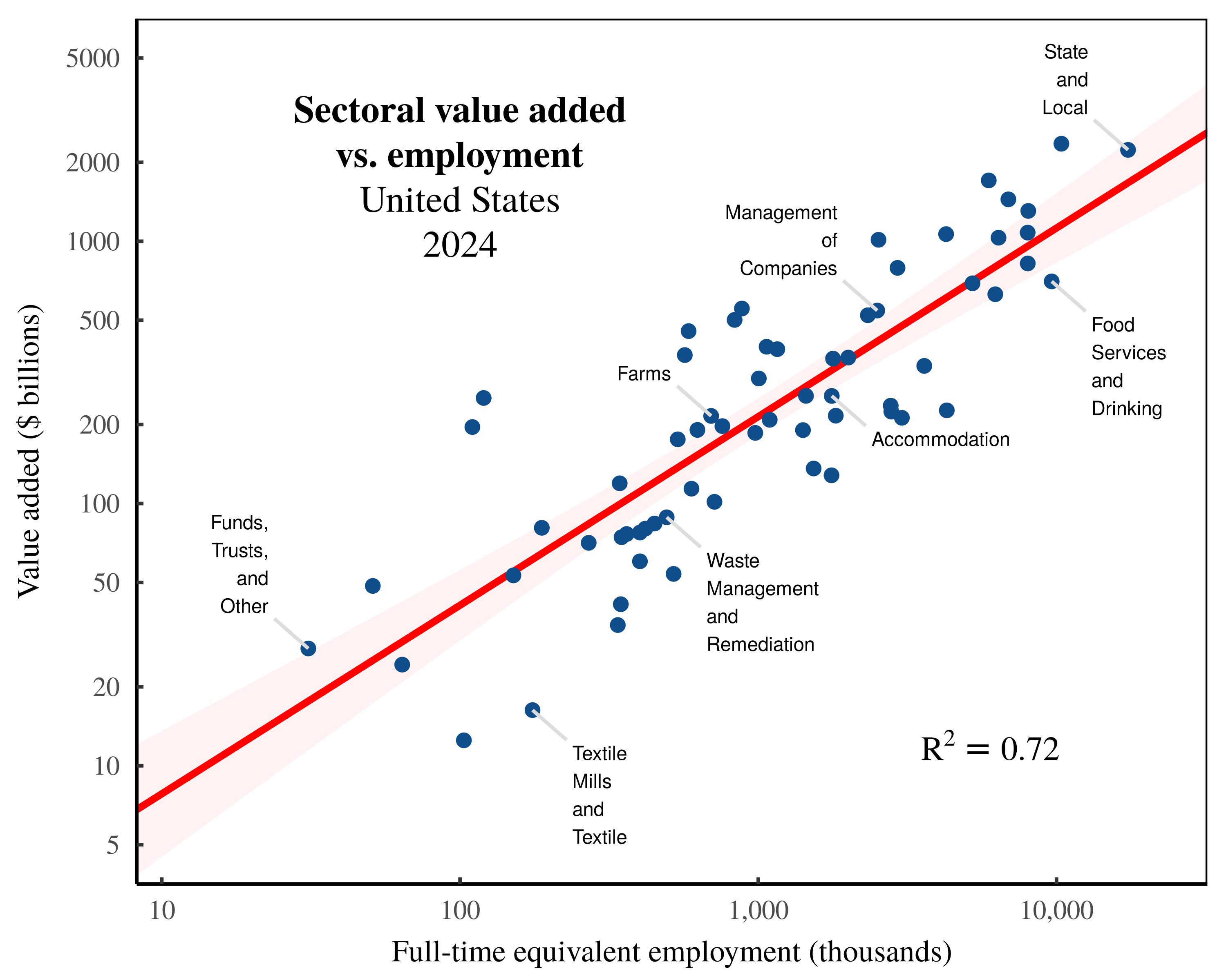Figure 1: Sectoral value added vs. employment in the United States.

Each point indicates a US sector in 2024. The vertical axis shows sectoral value added, while the horizontal axis shows full-time equivalent employment. Note the log scale on both axes. For data sources, see the Appendix.

---

Looking at Figure 1, the relation between employment and value added is quite tight. The question is, why? When answering this question, we face two options. The first option is to remain in the realm of metaphysics. Onto employment, we impose the concept of ‘labor value’. Then we suppose that through a series of unmeasured transformations, these values get transformed into the dollar value of ‘output’. In short, we close our minds and pretend to see invisible processes which remain unmeasured.

In contrast, the second option is to realize that in Figure 1, we are dealing with a bookkeeping relation, governed by predefined accounting identities. As such, the correlation between sectoral employment and sectoral value added is unsurprising, unremarkable, and says nothing about the validity of Marxist theory.

Taking this second path, let’s dive into the world of national accounting identities. We’ll begin by noting that ‘value added’, \footnotesize y , is defined to be the sum of labor compensation, \footnotesize l , and pretax capitalist income, \footnotesize k :

y = l + k (1)

Brief aside. Note that the jargon attached to Equation 1 reveals how mainstream economists misunderstand their bookkeeping. In their minds, labor and capital are both ‘factors of production’ which ‘add value’ to raw ingredients. Unfortunately, the value ‘inherent’ in this transformation is forever unobservable. And so economists simply transmogrify capital and labor income into the ‘value added’ they cannot measure. Ignoring this metaphysical alchemy, Equation 1 is simply a statement of double-entry bookkeeping. By definition, labor income and pretax capitalist income sum to the aggregate quantity, \footnotesize y , which by convention, is called ‘value added’.²

Continuing with more accounting identities, note that sectoral labor costs, \footnotesize l , are by definition, the product of full-time-equivalent employment, \footnotesize E , multiplied by the average sectoral wage, \footnotesize \bar{w} :

l = E \cdot \bar{w} (2)

Given this identity, it follows that ‘valued added’, \footnotesize y , is a function of employment, \footnotesize E :

y = E \cdot \bar{w} + k (3)

Looking at Equation 3, it is what I call a preordained noise function. That is, if we correlate value added with employment, Equation 3 predefines the statistical noise that we will observe. By definition, this noise is driven by cross-sector variation in the average wage, \footnotesize \bar{w} , and by cross-sector variation in pretax capitalist income, \footnotesize k . So to the extent that these quantities are fairly stable across sectors, we will observe a tight relation between \footnotesize y and \footnotesize E . The upshot of this thinking is that when we correlate ‘value added’ with employment, it is the noise in the relation that is of scientific interest. That’s because this noise tells us about cross-sector variation in wages and capitalist income — variation that is worth understanding.

Returning to Marxist metaphysics, notice that its effect is to distract us from the scientific content of the data. Our metaphysical thinking rationalizes the lack of noise in a bookkeeping correlation, whereas it is the noise itself that is worth studying.

Marxist alchemy option two: measure labor income and call it ‘labor value’

Continuing to think about Marxist metaphysics, sectoral employment is an incomplete measurement of ‘labor value’ for several reasons. First, to capture Marx’s theory, we should track the full web of embodied labor required to produce economic ‘output’. So in this sense, direct employment is a partial measure of ‘labor value’. Second, Marx insisted that ‘labor value’ should account for the different abilities of different workers.

It’s here that we get to the core metaphysical content of Marx’s theory. Looking at the work performed by specific people, Marx sees the machinations of a more abstract form of universal labor that accounts for different levels of skill. Hence, an hour of an neurosurgeon’s time is presumably worth more than an hour of a janitor’s time. Now, at least superficially, this thinking sounds reasonable. But on further inspection, it has bizarre consequences.

If ‘abstract’ labor time was a real-world entity, this would imply that workers with different skills become interchangeable. Thus, if an hour of a neurosurgeon’s time is worth eight hours of a janitor’s time, we should be able to walk into surgery, swap the neurosurgeon with eight janitors, and expect the same surgical outcome. Clearly, this swap is absurd, which is why Marxists are careful to differentiate between concrete labor (which is observable, but not interchangeable) and abstract labor (which is unobservable, but theorized to be universally interchangeable). Since Marxists place their hopes on the unobservable quanta of abstract labor, we can tell that we are dealing with metaphysics.

Still, we can pretend to observe this quanta by imposing it onto something we can measure, which is labor income. Looking at workers with different wages, we suppose that their wages reveal their skill at creating value. As it happens, this alchemy is standard practice in neoclassical economics, where wages are treated as a proxy for ‘productivity’ (Fix, 2018). But when Marxists use wages as a proxy for skill, they use a different name. Multiplying employment by the wage rate, we get the Marxist metaphysical quantity known as ‘skill-adjusted labor time’.

Returning to the United States, we find that across sectors, ‘skill-adjusted labor time’ correlates strongly with sectoral value added. Figure 2 shows the relation in 2024. (Note that this correlation is tighter than the employment relation shown in Figure 1.)

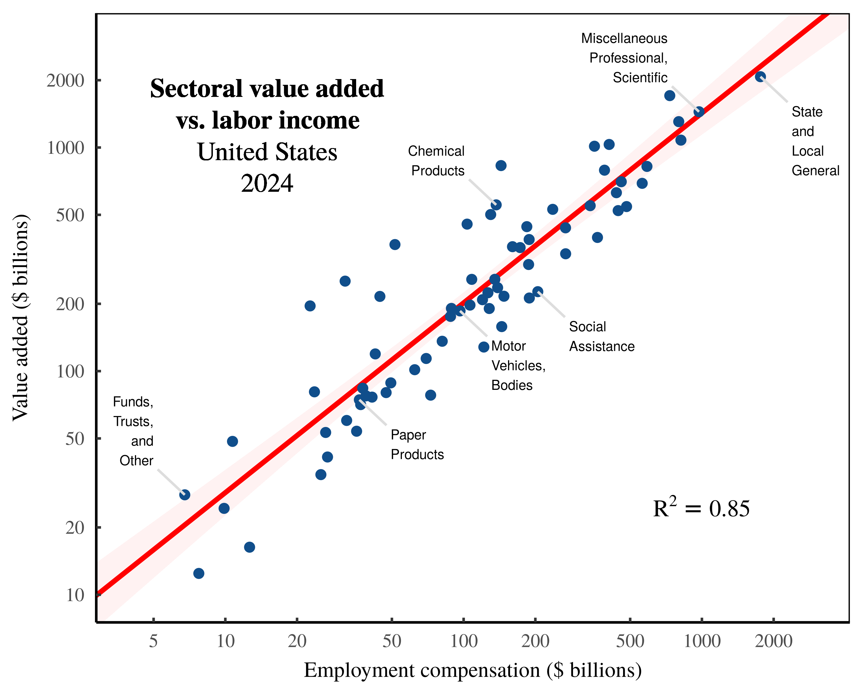Figure 2: Sectoral value added vs labor income in the United States.

Each point indicates a US sector in 2024. The vertical axis shows sectoral value added, while the horizontal axis shows sectoral labor income. Note the log scale on both axes. For data sources, see the Appendix.

---

Looking at the evidence in Figure 2, we again have two options. We can either double down on our metaphysics, or we can realize that we are dealing with another bookkeeping correlation. Taking the latter option, we realize that our supposed measurement of ‘skill-adjusted labor time’ is simply an observation of labor costs, \footnotesize l . It consists of the product of employment, \footnotesize E , times the average wage, \footnotesize \bar{w} :

l = E \cdot \bar{w} (4)

Labor costs, in turn, are tied to value added, \footnotesize y , by a bookkeeping identity:

y = l + k (5)

So what we have, with Equation 5, is another preordained noise function. If we correlate labor costs, \footnotesize l , with ‘value added’, \footnotesize y , we know before we even look at the data that the statistical noise will be driven by cross-sector variation in pretax capital income, \footnotesize k . If this variation is fairly small, then our correlation will be tight, just as it is in Figure 2.³

Again, the scientifically interesting feature of our bookkeeping correlation is the statistical noise, which tells us about variation in the sectoral distribution of income. And again, Marxist metaphysics distracts us from this intriguing feature of the real world.

Marxist alchemy option three: measure total (direct + indirect) labor costs and call it ‘labor value’

Let’s now finalize our decent into Marxist metaphysics. The missing piece of our metaphysical puzzle is the measurement of wholesale embodied labor values — a measurement that tracks not just the direct ‘skill-adjusted labor’ in each sector, but also includes the full web of labor value that is embodied in the exchange of commodities between sectors.

Here, our metaphysics is helped by techniques developed by mainstream economists. As part of the national accounts, economists construct ‘input-output’ tables that track the web of embodied inputs used in each sector. As such, we can use these methods to make a ‘definitive’ calculation of total sectoral labor values. The technique behind this definitive calculation was (to my knowledge) first proposed by Anwar Shaikh (1984).

Here, I will skip the details and cut to the results. If we use Shaikh’s method, we find an extremely tight correlation between imputed total labor values and the gross value of sectoral output. Figure 3 shows the relation across US sectors in 2024.

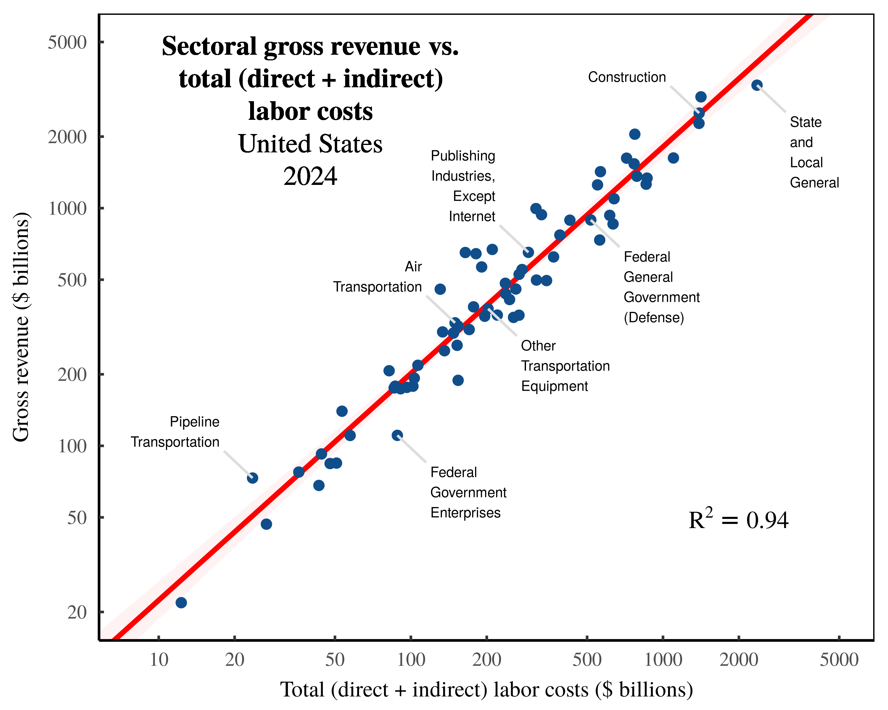Figure 3: Sectoral gross revenue vs. total (direct + indirect) labor costs in the United States.

Each point indicates a US sector in 2024. The vertical axis shows sectoral gross revenue, while the horizontal axis shows total sectoral labor costs — the sum of direct employment compensation plus the indirect expenses ultimately paid to workers at large. Note the log scale on both axes. For data sources, see the Appendix.

---

That’s the metaphysical story, anyway. Back in the real world, Figure 3 shows yet another bookkeeping correlation, but one which takes more effort to unpack. The starting point is that we are again taking the Marxist metaphysical concept of ‘skill-adjusted labor time’ and imposing it onto the measurement of labor costs. The more confusing part is that we are also adding the metaphysics of ‘input-output’ analysis.

Despite what their name implies, ‘input-output’ tables track neither ‘inputs’ nor ‘outputs’. (This naming convention is a classic example of metaphysical alchemy.) What these tables do is track purchases and sales across sectors. Which is to say that when economists use these tables to track ‘inputs’, what they are actually doing is tracking intersectoral expenses. Hence when Shaikh uses input-output data to calculate the ‘total skill-adjusted labor inputs’ to each sector, he is actually measuring the total expenses which are eventually paid out to workers.

Let’s now discuss the bookkeeping involved in this calculation. To start, when economist speak about ‘gross output’, they are imposing their metaphysics onto the measurement of gross revenue, \footnotesize g . And gross revenue, in turn, is defined by the following identity:

g = l + k + e (6)

Here, \footnotesize l is the money paid directly to workers, \footnotesize k is the pretax income received directly by capitalists, and \footnotesize e represents the ‘intermediate expenses’ paid to other firms.⁴ Now, according to the rules of double-entry bookkeeping, one person’s expenses must eventually become another person’s income. As such, if we followed a firm’s expenses as the money flows outwards across society, we know that each dollar spent must eventually land in one of two places. Either the money gets paid to a worker, or it gets paid to a capitalist.⁵ Given these two destinations, it follows that in Equation 6, we can decompose the expense term, \footnotesize e , as follows:

g = l + k + e_l + e_k (7)

Here, \footnotesize e_l represents the intermediate expenses that are eventually paid to labor. And \footnotesize e_k represents the intermediate expenses that eventually flow to capitalists. Now, without changing the mathematics, we can regroup terms by their income type:

g = ( l + e_l ) + ( k + e_k ) (8)

Then we can exercise our right to create accounting definitions. Let \footnotesize l_t be the sum of direct and indirect labor costs:

l_t = l + e_l (9)

And let \footnotesize k_t be the sum of direct and indirect pretax capitalist income:

k_t = k + e_k (10)

With our bookkeeping complete, we can now restate our gross-revenue identity. Gross revenue, \footnotesize g , equals the sum of total labor income, \footnotesize l_t , plus total pretax capitalist income, \footnotesize k_t :

g = l_t + k_t (11)

Looking at Equation 11, we have deduced yet another preordained noise function. If we correlate total labor costs with gross revenue (as in Figure 3), we know the source of the statistical noise before we even gaze at the data. The noise is generated by cross-sector variation in total pretax capitalist income, \footnotesize k_t .

The catch, however, is that the identity in Equation 11 hides some fairly complex calculations used to track indirect costs. As such, it takes some effort to understand the statistical noise function being evoked. I will unpack this algebra in Part 2. But first, let me indulge in some satirical metaphysics.

Testing the capitalist theory of value

Perhaps the most important feature of metaphysical alchemy is that it operates in the direction we choose. In other words, Marxists are free to take a bookkeeping correlation and impose their metaphysics onto it. But everyone is entitled to do the same procedure with whatever metaphysics they like.

As a satirical demonstration of this principle, let me now present a ‘test’ of the ‘capitalist theory of value’. In this theory, we suppose that it is capitalist owners who create all value. The story goes something like this: while dozing in their private jets, billionaires like Elon Musk and Jeff Bezos are busy generating vast sums of value for society. Of course, we cannot observe this ‘capitalist value’. But we can impose the metaphysical idea of this value onto the thing we do observe, which is capitalist income.

As an illustration of this procedure, let’s now look at the inversion of Anwar Shaikh’s method. In this inversion, we take Shaikh’s empirical method for calculating total ‘labor values’, and we swap out references to ‘labor’ with references to ‘capital’. (Since we are dealing with bookkeeping calculations, the swap is extremely simple.) Then, we grab some US data and test our capitalist theory of value. Lo and behold, we find that imputed ‘capitalist values’ correlate tightly with the value of sectoral ‘output’. Figure 4 shows the relation across US sectors in 2024.

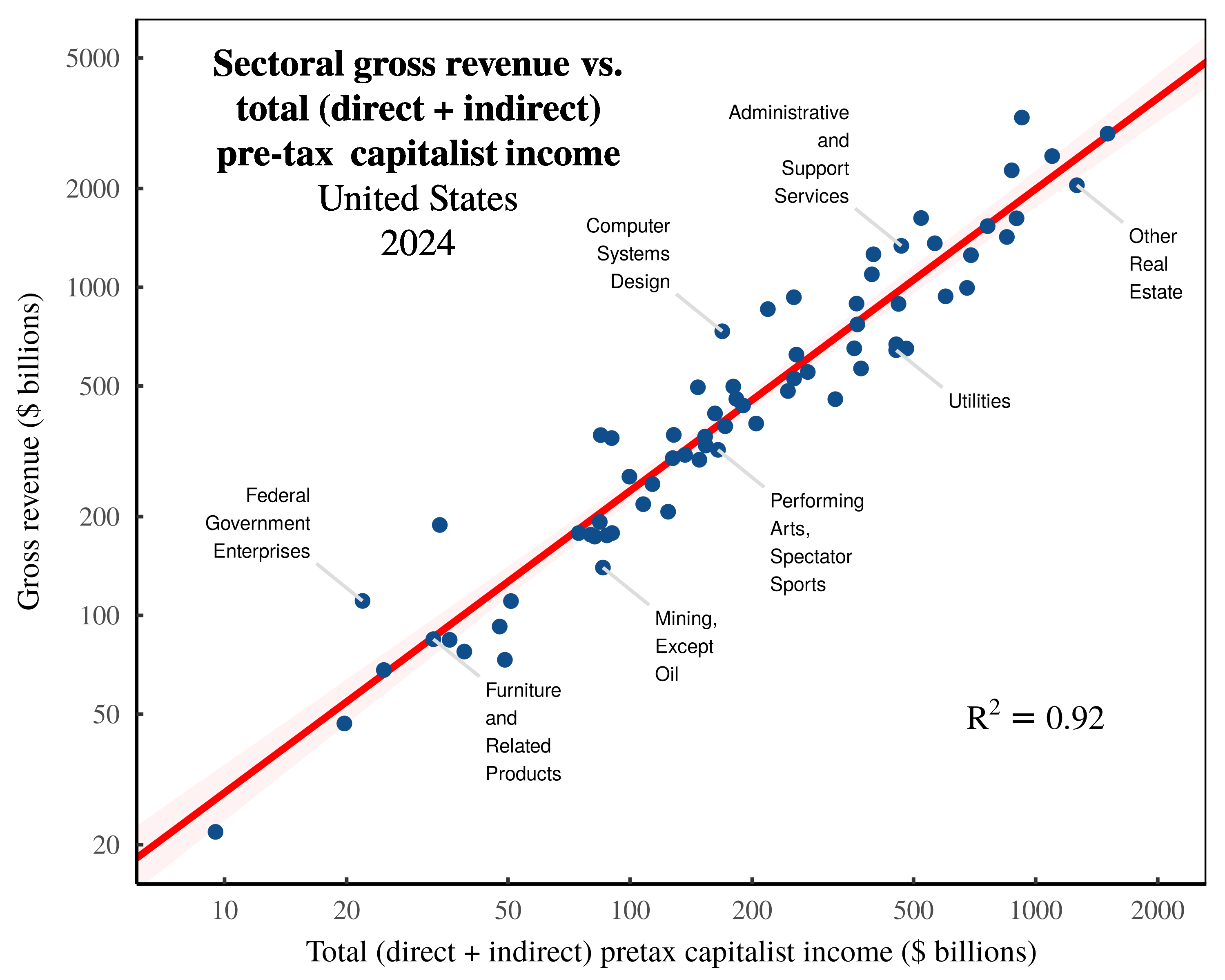Figure 4: Sectoral gross revenue vs. total (direct + indirect) pretax capitalist income in the United States.

Each point indicates a US sector in 2024. The vertical axis shows sectoral gross revenue, while the horizontal axis shows total pretax capitalist income — the sum of direct pretax capitalist income in each sector, plus the indirect expenses ultimately paid to capitalists. Note the log scale on both axes. For data sources, see the Appendix.

---

Backing away from this satire, what Figure 4 actually shows is the bookkeeping relation that is logically contained within Figure 3. Let’s unpack this statement.

In Figure 3, I used (an untransmogrified version of) Shaikh’s empirical method to measure the total (direct + indirect) labor costs in each sector. Now by definition, the conjugate of these total labor costs is the total pretax income flowing to capitalists. That is, by definition, total labor costs, \footnotesize l_t , plus total pretax capitalist income, \footnotesize k_t , sum to sectoral gross revenue, \footnotesize g . (See Equation 11.) Here, then, is the logical conclusion. If total labor costs correlate tightly with sectoral gross revenue, then total pretax capitalist income should also correlate tightly with sectoral gross revenue.⁶ Such is the nature of double-entry bookkeeping, which renders the pattern in Figure 4 unsurprising.

To summarize, we have learned that double-entry bookkeeping ensures that expenses relate to income. (These two quantities are literally two sides of the same equation.) Now, to the extent that we impose a simple classification scheme onto expenses, we will find that categories of expenses correlate tightly with total income.⁷ The logical limit is when all expenses are lumped into a single category, in which case, expenses are simply a restatement of revenue.⁸ In the case of two categories of expenses — money flowing to labor and money flowing to capitalists — the situation is only slightly less circular. As Figures 3 and 4 demonstrate, we still find remarkably tight relations between revenue and expenses.

The lesson is that when we study bookkeeping identities, we understand that Figure 3 and Figure 4 are two sides of the same coin. And yet Marxists invariably point to the labor side of this equation, and ignore the capitalist side. Why? The reason obviously has nothing to do with science. Marxists focus on labor costs because it is convenient for their metaphysics. But the truth is that the bookkeeping itself cares nothing for Marxist dogma; indeed the same data will happily permit a complete inversion of Marxist theory. Which of course, is why metaphysics is not science.

Part 2: Deconstructing the Shaikh method

At this point, I’ve concluded my high-level discussion of Marxist metaphysical alchemy. For the remainder of the paper, I will dive into the details of Anwar Shaikh’s empirical method for ‘testing’ the labor theory of value.

My goal is to explain what exactly Shaikh measures, why this measurement is scientifically interesting, and how this measurement is subverted for metaphysical purposes. My investigation builds on Sabatino’s analysis, which demonstrates that Shaikh’s empirical method seems to ‘work’ (as in ‘verify’ the labor theory of value) even when fed nonsense data. The reason this happens, I will argue, is that Shaikh’s method amounts to a Rube-Goldberg device for transforming noise in the labor share of income into noise in ‘labor values’.

From Marx to Sraffa … to national bookkeeping

For decades, Anwar Shaikh has argued that Marx’s labor theory of value could be re-interpreted in terms of Sraffa’s analysis of commodity production (Shaikh, 1984, 1998, 2016).

The backstory is that in his seminal book Production of Commodities by Means of Commodities, Piero Sraffa proposed analytic methods for studying the relation between commodity inputs, outputs, and prices (1960). This method, Shaikh argues, can be used to solve the Marxist problem of tracking the labor inputs to production, and thus allows for a rigorous ‘test’ of Marx’s labor theory of value.

The second backstory is that Sraffa’s analysis of commodity production is every bit as metaphysical as Marx’s labor theory of value.⁹ In the real world, we never know the complete list of commodities needed to produce other commodities. Indeed, economists never even attempt to construct such lists. But what economists do construct is bookkeeping tables, which track revenue and expenses. As a result, when Shaikh claims to implement Sraffian methods, what he is actually doing is imposing Sraffian metaphysics (of commodity ‘inputs’ and ‘outputs’) onto the analysis of monetary transactions. Of course, mainstream economists play the same game, which is why such metaphysics generally go unquestioned.

What is unfortunate here is that when stripped of its metaphysics, Shaikh’s accounting method is legitimately useful. Indeed, it highlights how the national accounts can be used dissect the financial structure of capitalism. Given this legitimate use, let’s dive into the details of Shaikh’s calculation.

Tracking transaction sprawl

The entirety of Shaikh’s (untransmogrified) empirical method can be stated in a single equation. For every sector, Shaikh’s method calculates total labor costs, \footnotesize l_t , as follows:

\boldsymbol{ l_t } = \left[ \left( \boldsymbol{l} \oslash \boldsymbol{g} \right) \left( \boldsymbol{I} - \boldsymbol{A} \right)^{-1} \right] \circ \boldsymbol{g} (12)

For the rare reader who understands the machinations of linear algebra, everything that follows is contained within Equation 12. But for everyone else (including myself), the algebra in Equation 12 is opaque, and requires an extended exposition to be comprehensible. For that reason, I won’t bother to define the terms in this equation, because they only make sense in hindsight, after we know what is being calculated.

To understand Equation 12, the best place to start is with the question being posed, which is this: if a firm spends money (at large), what portion of that money eventually gets paid to workers? Shaikh’s method answers this question, not for individual firms, but for the groups of firms which we call ‘sectors’.

Zooming out to the big picture, governments could (if they were feeling invasive) compel all firms to publish their books to a central repository, in which case we could construct a wildly detailed database of inter-firm and intra-firm transactions. Suffice it to say that governments do not compel such reporting, but instead, appeal to a more roughshod sampling method, in which they estimate transactions between large-scale groups of firms. These tables are then mislabeled as ‘input-output’ accounts, but I will ignore this dubious convention here.

To get a sense for how intersectoral transaction tables work, let’s turn to Figure 5. Here, I have created a hypothetical table which tracks transactions among four sectors. Each cell reports a transaction, with the label indicating the sectoral participants, and color showing the relative transaction size. (For example, the label \footnotesize 1 \rightarrow 2 indicates that money is sent from Sector 1 to Sector 2.)

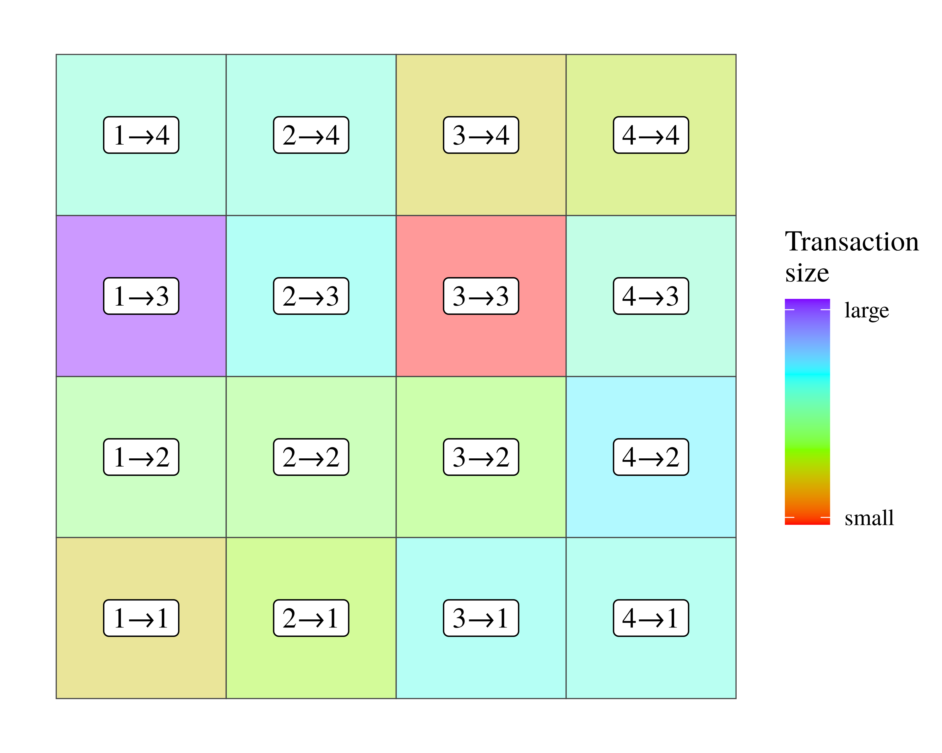Figure 5: An example of an intersectoral transaction table among four sectors.

In this table, each cell denotes a monetary transaction between sectors. Labels indicate the sectoral participants, and the direction of the transfer. Color shows the size of the transaction.

---

Looking at this transaction table, the (untransmogrified) goal of Shaikh’s method is to follow money as it weaves across sectors, and to deduce where it lands. For example, money leaving Sector 1 might head to Sector 3. Once there, the money could be re-spent to Sector 2, where it is then sent back to Sector 3. Such a transaction path would look like this:

\displaystyle 1 \rightarrow 3 \rightarrow 2 \rightarrow 3 \rightarrow \ldots

Of course, many other transaction paths are possible. And therein lies the conceptual problem with analyzing intersectoral transactions. Technically, the web of transactions is unbounded, meaning money can (in principle) circulate indefinitely among sectors. As such, it would seem that there are infinitely many transaction paths to be studied.

Returning to Equation 12, the matrix term \footnotesize \left( \boldsymbol{I} - \boldsymbol{A} \right)^{-1} exists to solve this infinite transaction problem. First proposed by Wassily Leontief (1953), this ‘Leontief inverse matrix’ is an algebraic method for inferring the limiting behavior of a network of unbounded transaction.¹⁰ Now, the nice thing about the Leontief inverse matrix is that it is easy to implement with a computer. But the downside is that the meaning of the calculation is obscured within the intricacies of linear algebra. For that reason, I find it helpful to plot a bounded version of of the calculations contained within this matrix.

Figure 6 shows an example of what I call ‘transaction sprawl’. The idea here is that we are following money as it leaves a given sector and enters the network of intersectoral transactions. For simplicity, I’ve visualized the four-sector model shown in Figure 5. (Larger models quickly get out of hand.) In Figure 6, we track money as it leaves Sector 1. When the money is received by another sector, it is spent again. During each iteration of re-spending, the transaction network sprawls outwards, adding an expanding number of transaction paths.

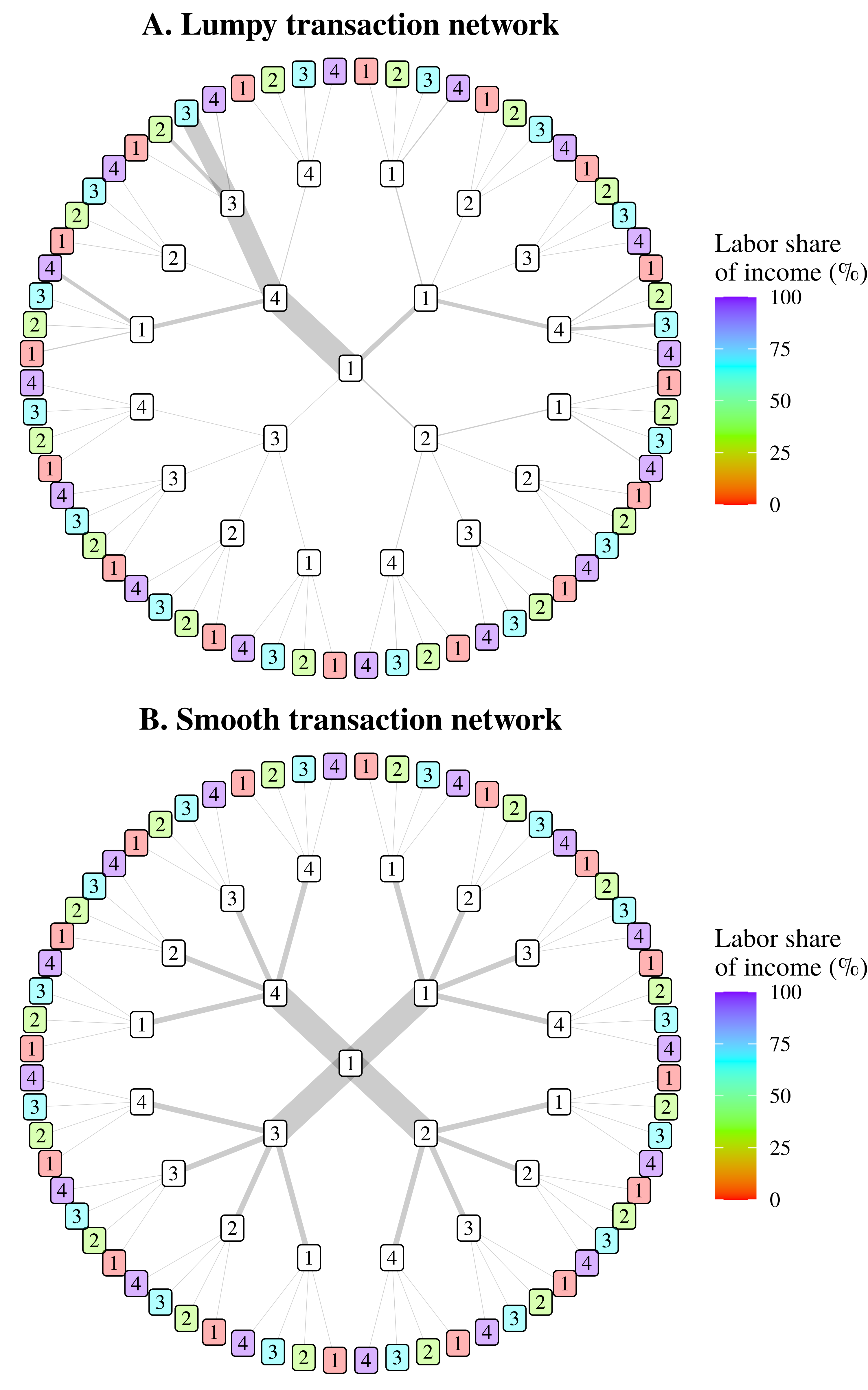Figure 6: Visualizing intersectoral transaction sprawl.

This chart illustrates a truncated version of the math contained within the Leontief inverse matrix, as used by Anwar Shaikh to track indirect labor expenses. Using the four-sector model shown in Figure 5, we track expenses as they leave Sector 1. When money is received by a new sector, it is re-spent, leading to a growing network of ‘transaction sprawl’. Here, I have stopped the sprawl after three transactions. Color in the end nodes indicates the labor share of income in each destination sector, which is used to calculate the labor portion of intermediate expenses. Lastly, note that the top panel shows a ‘lumpy’ transaction network, in which most of the money travels down a few paths. In contrast, the bottom panel shows a ‘smooth’ transaction network, in which money flows equally down all paths.

---

Now in principle, this transaction sprawl can grow indefinitely. But for illustration purposes, I’ve stopped the sprawl after three iterations. At this point, patterns are already evident. Backing up a bit, in Figure 6, the line thickness indicates the volume of money heading down a given transaction path. Looking at Figure 6A, for example, we see that much of the money heads down the path \footnotesize 1 \rightarrow 4 \rightarrow 3 \rightarrow 3 . (We will return to this lumpy transaction behavior in a moment.) We also see that after each iteration of re-spending, the volume of money arriving at each end-node tends to exponentially decrease. It is because of this decrease that our unbounded network sprawl has bounded behavior.

Looking at the transaction sprawl in Figure 6, notice that despite the growing complexity of the transaction network, there are still only four sectors in which the money can ‘land’. (The outer nodes of the network repeat the same four sectors a growing number of times.) Because of this discrete behavior, we can express the limiting behavior of our network sprawl in terms of a weighted average. But first, I should explain why the outer nodes are colored.

In Figure 6, the color of the outer nodes indicates the (hypothetical) labor share of income in each sector. The idea here is that when implementing Shaikh’s method, we are interested in the subset of ‘intermediate expenses’ which ultimately get paid to workers. Looking at a particular transaction path, we can calculate this subset by taking the money that travels down a given path, and multiplying it by the labor share of income in the destination sector. For example, suppose that $10 billion worth of intermediate expenses travels down the path \footnotesize 1 \rightarrow 4 \rightarrow 3 \rightarrow 3 . Looking at Sector 3, we see that its labor share of income is 75%. Hence, of the $10 billion worth of intermediate expenses arriving in Sector 3 (via this particular path), $7.5 billion gets paid to workers.

To compute the labor portion of our full web of transaction sprawl, the task is to repeat this calculation for every path to every endpoint sector. Clearly, the job is lengthy and complicated. However, it turns out that the results of this calculation can be summarized with a simple equation.

Let \footnotesize e_l be the subset of intermediate expenses (leaving our center node) which are ultimately paid to workers in other sectors. To calculate this quantity, we take a weighted sum of the labor share of income, \footnotesize L , in each sector \footnotesize i . The weights of this sum, \footnotesize e_i , are the total intermediate expenses sent from the central node which arrive in sector \footnotesize i :

e_l = \sum_{i=1}^n e_i \cdot L_i (13)

If we then divide both sides of this equation by \footnotesize e (the total intermediate expenses spent by our central node), our equation becomes a weighted average:

\frac{e_l}{e} = \frac{ \sum_{i=1}^n e_i \cdot L_i }{e} (14)

Now, the question is whether this computational summary is of any help. And in general, the answer is ‘no’. In other words, the numerical content of Equation 14 lies in the weighting terms, \footnotesize e_i , which are a complicated consequence of the specific transaction network. There is, however, an exception, which I have visualized in Figure 6B.

In contrast to Figure 6A, which visualizes a ‘lumpy’ transaction network in which most of the money heads down a few transaction paths, Figure 6B illustrates a ‘smooth’ transaction network. In this latter scenario, money flows equally down all transaction paths. Because of this smooth behavior, the weighting terms in Equation 14 become trivial to calculate. Each weighting term, \footnotesize e_i , collapses to \footnotesize e/n , where \footnotesize n represents the number of sectors. As a consequence, Equation 14 reduces to an unweighted average of the cross-sector labor share of income:

\lim_{e_i \rightarrow e/n } ~ \frac{e_l}{e} = \frac{ \sum_{i=1}^n L_i }{n} = \overline{L} (15)

In this ‘smooth transaction limit’, we can predict the labor portion of intermediate expenses without knowing anything about specific transactions. Or put another way, in the smooth transaction limit, a sector’s indirect labor costs, \footnotesize e_l , become a simple product of the average cross-sector labor share of income:

e_l = e \cdot \overline{L} (16)

Thinking about this equation, the pertinent question is whether the smooth transaction limit says anything about the real world. Surprisingly, the answer is yes.

The ‘smooth’ transaction approximation

In the limit that intersectoral transactions are perfectly smooth, the labor portion of intermediate expenses becomes an exact function of the cross-sector average labor share of income. What I want to do now is imagine that we slowly add ‘lumps’ to our intersectoral transactions. As we do, our smooth transaction limit goes from being an identity to being an approximation:

e_l \approx e \cdot \overline{L} (17)

Here is the interesting question: How lumpy do transactions have to be before this approximation becomes useless? Surprisingly, the answer is ‘extremely lumpy’. But I am getting ahead of myself.

To answer our question, we must first define a way to measure transaction ‘lumpiness’. I will use the Gini index, which is a measure of inequality that varies from 0 (perfect equality) to 1 (perfect inequality). Looking at a transaction network, ‘smooth’ transactions will have a low Gini index, while ‘lumpy’ transactions will have a high Gini index. Next, I need to clarify the relevant transactions to be measured. To quantify transaction lumpiness, I will calculate the Gini index on the columns of the ‘direct requirements table’. (In Equation 12, this table is denoted as \footnotesize \boldsymbol{A} ). Then I’ll average the results to get a single measure for transaction ‘lumpiness’ across all sectors.¹¹

As a thought experiment, let’s first examine the smooth transaction approximation in a 1000-sector model, characterized by random intersectoral transactions (sampled from a lognormal distribution). In this model, I will tailor transaction ‘lumpiness’ to have a Gini index of exactly 0.5. (For context, this Gini index corresponds to the level of US income inequality in the 1980s.)

With my simulated data, I apply Equation 12 to calculate the total labor costs, \footnotesize l_t , in each sector. From there, I calculate indirect labor costs, \footnotesize e_l , by subtracting direct labor costs, \footnotesize l , from total labor costs:

e_l = l_t - l(18)

Next, I measure how each sector’s indirect labor costs, \footnotesize e_l , scale with intermediate expenses, \footnotesize e . Since the absolute values of \footnotesize e_l and \footnotesize e are uninteresting, I normalize these values against sectoral gross revenue, \footnotesize g :

\frac{e_l}{g} \sim \frac{e}{g} (19)

Figure 7A illustrates this comparison for my 1000-sector model. (Here, each point represents a sector.) For reference, the red line shows the smooth transaction approximation, in which indirect labor costs scale perfectly with intermediate expenses, with a slope of \footnotesize \overline{L} . What’s important is here is that despite the significant lumpiness of the intersectoral transactions, the smooth transaction approximation remains an accurate substitute for the full-scale math of Shaikh’s method.

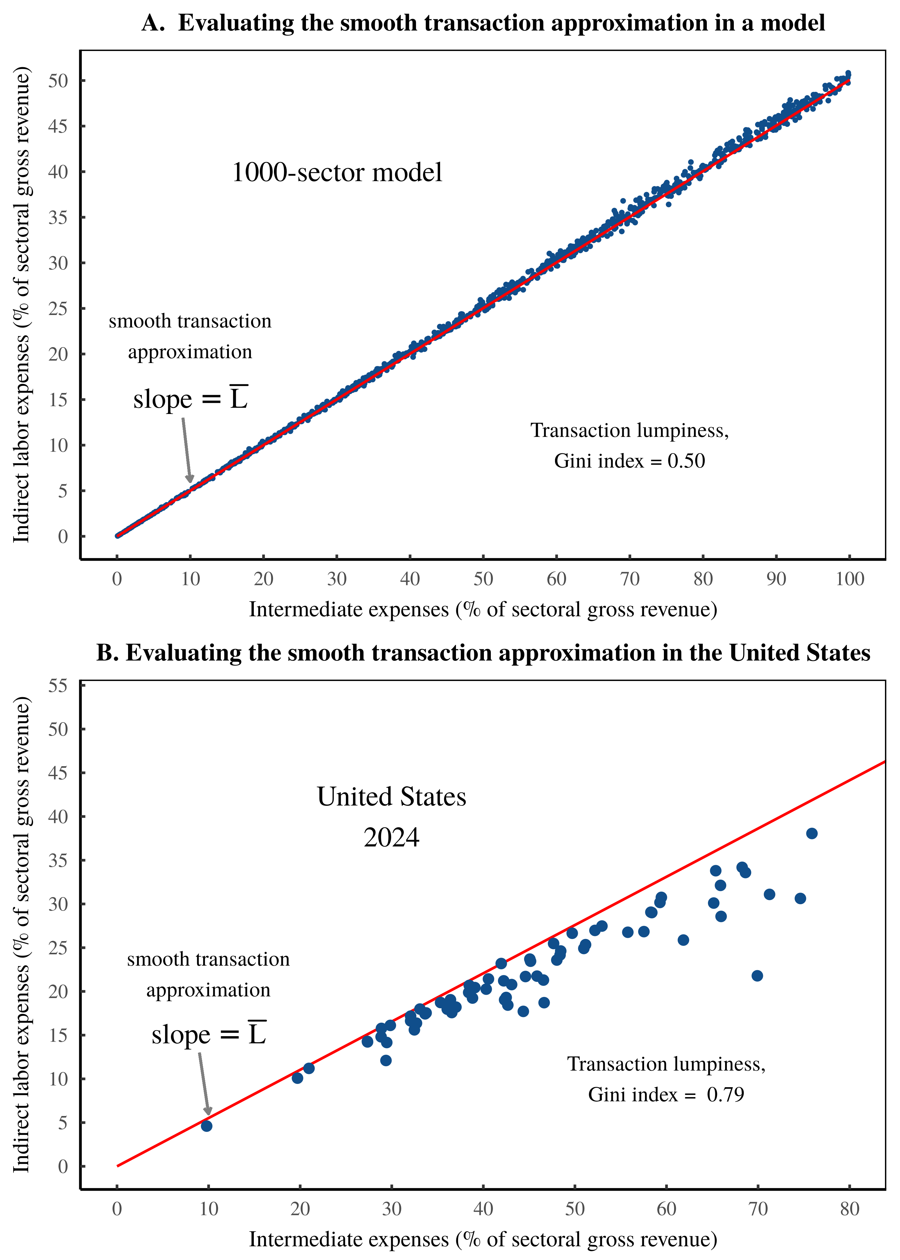Figure 7: Testing the smooth-transaction approximation.

Using the Shaikh method, this chart tests the ‘smooth transaction approximation’ — the idea that across sectors, indirect labor costs scale as a simple function of intermediate expenses, where the slope of this relation is the cross-sector average labor share of income, \footnotesize \overline{L} . In each panel, the vertical axis shows indirect sectoral labor costs, normalized against sectoral gross revenue. The horizontal axis shows sectoral intermediate expenses, also normalized against gross revenue. Each point represents a sector. Panel A shows the behavior of a 1000-sector model in which intersectoral transactions are random numbers. Panel B shows the behavior across US sectors in 2024. Note that the accuracy of the smooth transaction approximation is determined by the ‘lumpiness’ of intersectoral transactions, which I have measured here using the Gini index. The lumpier these transactions, the less accurate the approximation. For details and data behind this chart, see the Appendix.

---

Turning to the real world, let’s look at US intersectoral transactions in 2024. Here, we find an even lumpier set of transactions, in which the Gini index is 0.79. (For context, this Gini index corresponds to the level of US wealth inequality in the early 1990s.) Despite this significant ‘lumpiness’, the smooth transaction limit remains a reasonable approximation for the full-scale math of Shaikh’s method. Figure 7B shows the pattern.¹²

The lesson here is that we now grasp the rough ‘meaning’ of Equation 12. To reiterate, this equation defines the (untransmogrified) math behind Shaikh’s calculation of the total expenses flowing to workers, \footnotesize l_t . By definition, these costs consist of the sum of direct labor costs, \footnotesize l , plus the subset of intermediate expenses eventually paid to workers, \footnotesize e_l :

l_t = l + e_l (20)

Using the smooth transaction approximation, we can estimate these total labor costs with zero knowledge of intersectoral transactions. All we need to know is each sector’s intermediate expenses, \footnotesize e , and the average cross-sector labor share of income, \footnotesize \overline{L} :

l_t \approx l + e \cdot \overline{L}(21)

Given the complexity of Shaikh’s method, it is somewhat surprising that it can be approximated by such a simple function.

Preordained noise in the Shaikh method

With our smooth-transaction approximation in hand, we are now ready to study the preordained noise in Shaikh’s ‘test’ of the labor theory of value. Absent the Marxist metaphysics, Shaikh’s method consists of a straightforward correlation; it compares sectoral gross revenue, \footnotesize g , with total (direct + indirect) labor costs, \footnotesize l_t :

g \sim l_t (22)

To understand the preordained noise in this comparison, it is helpful to restate Equation 22 as a form of autocorrelation. When we correlate \footnotesize g with \footnotesize l_t , we are observing the perfect correlation between \footnotesize g and itself, multiplied by variation in the ratio \footnotesize l_t /g :

g \sim \left( \frac{l_t}{g} \right) \cdot g (23)

My goal now is to understand the noise term, \footnotesize l_t / g . To get started, recall that by definition, total labor costs, \footnotesize l_t , consist of direct labor costs, \footnotesize l , plus the subset of intermediate expenses ultimately paid to workers, \footnotesize e_l :

l_t = l + e_l (24)

In rough terms, we learned (in the previous section) that indirect labor costs, \footnotesize e_l , can be estimated using the smooth transaction approximation, in which \footnotesize e_l \approx e \cdot \overline{L} . Using this approximation, our correlation becomes:

g \sim \left( \frac{l + e \cdot \overline{L} }{g} \right) \cdot g (25)

Peering ahead, we will end up repeatedly dividing by the gross revenue term, \footnotesize g . To unclutter the math, I will introduce a subscript notation for this division. Going forward, anytime you see the \footnotesize g subscript, it indicates dividing by \footnotesize g . For example, \footnotesize l_g = l / g . And \footnotesize e_g = e / g . Introducing this notation, we can rewrite Equation 25 as:

g \sim \left(~ l_g + e_g \cdot \overline{L} ~ \right) \cdot g (26)

Looking at Equation 26, I would like to replace the intermediate expense term, \footnotesize e_g , with terms for labor income. To do that, Box 1 takes a brief detour into the land of national accounting identities.

Using the results from Box 1 (Equation 38), we can now replace the intermediate expenses term, \footnotesize e_g , in Equation 26. The substitution gives:

g \sim \left( l_g + \frac{ L - l_g }{L} \cdot \overline{L} \right) \cdot g (39)

To summarize, Equation 39 it tells us that Shaikh’s ‘test’ of the labor theory of value consists of correlating sectoral gross revenue, \footnotesize g , with itself, with added statistical noise provided by \footnotesize \sigma :

g \sim \sigma \cdot g (40)

From national accounting identities, we now know that the statistical noise, \footnotesize \sigma , is preordained, and can be approximated by the following function:

\sigma \approx l_g + \frac{ L - l_g }{L} \cdot \overline{L} (41)

The circular limit

Looking at Equation 41, my contention is that cross-sector variation in our statistical noise, \footnotesize \sigma , is driven by cross-sector dispersion in the labor share of income, \footnotesize L . To demonstrate this connection algebraically, let’s suppose that in each sector, the labor share of income is some perturbation, away from the cross-sector mean in the labor share of income, \footnotesize \overline{L} . Denoting this perturbation \footnotesize \epsilon , we can write:

L = \epsilon \cdot \overline{L} (42)

When we introduce this perturbation into Equation 41, our noise function becomes:

\sigma (\epsilon) \approx l_g + \frac{ \epsilon \cdot \overline{L} - l_g }{ \epsilon \cdot \overline{ L } } \cdot \overline{L} (43)

To demonstrate that our noise function is driven by \footnotesize \epsilon , we can see what happens as \footnotesize \epsilon approaches one. (This limit is a mathematical way of saying that the labor share of income becomes uniform across sectors.) In this limit, our noise function collapses to a constant — a constant that happens to equal the average labor share of income, \footnotesize \overline{L} :

\lim_{ \epsilon \rightarrow 1 } ~ \sigma (\epsilon) \approx l_g + \frac{ \overline{L} - l_g }{ \overline{ L } } \cdot \overline{L} ~=~ \overline{L} (44)

To summarize this journey into preordained noise, we can state that in the limit where the labor share of income is uniform across sectors, Shaikh’s ‘test’ of the labor theory of value reduces to a simple tautology. It correlates sectoral gross revenue, \footnotesize g , with a perfect transformation of itself:

g \sim \overline{L} \cdot g (45)

The corollary of this tautology, which I will investigate shortly, is that to the extent that the labor share of income is not identical across sectors, it is cross-sector income dispersion which drives the noise in Shaikh’s method.

A transmogrification interlude

At this point, it is worth bridging the gap between my presentation of Shaikh’s method, and Shaikh’s metaphysical articulation of (essentially) the same math.

To start, Shaikh presents his calculations in terms of ‘prices’. (He claims to relate ‘market prices’ to Marxian ‘direct prices’.) This language is metaphysical alchemy. In the real world, every input and output to Shaikh’s method is a measure of aggregate monetary value, which means that his method says nothing about commodity prices. So why the ruse? My guess is that it is wishful thinking. Shaikh would like to test Marx’s claim that labor values determine commodity prices. But since he cannot conduct such a test, he simply imposes the language of prices onto aggregate monetary value.

Next, Shaikh speaks of imputing ‘labor values’. But his measurement is actually a transmutation of total labor costs. Most of the heavy lifting here is done with Marxist rhetoric. But a lesser portion is done by a simple normalization trick. Shaikh’s imputed labor values, which I will call \footnotesize v , consist of a normalized version of total labor costs, \footnotesize l_t :

v = \mu \cdot l_t (46)

Now in Shaikh’s telling, the normalization constant, \footnotesize \mu , serves to ‘transform’ labor values into monetary value. (In Marxist jargon, \footnotesize \mu measures the ‘monetary expression of labor time’ — the amount of labor value embodied in each unit of currency.) The assumption here is that \footnotesize l_t measures labor values in units of socially necessary abstract labor time. To transform these units of time into units of money, we need to introduce a conversion constant, which is ostensibly \footnotesize \mu .

Back in reality, the variable \footnotesize l_t is in fact a measurement of labor costs. As such, there’s no need to convert units of time into units of currency, because we’re already dealing with a measurement of aggregate monetary value.¹³ In this light, Shaikh’s ‘transformation’ is a method for normalizing total labor costs so that they look more like gross revenue. Shaikh’s normalization constant, \footnotesize \mu , ensures that transmogrified labor costs sum to total gross revenue:

\mu \sum l_t = \sum g (48)

Metaphysics aside, the effect of this normalization is to shift the center of Shaikh’s preordained noise function, \footnotesize \sigma , such that it is centered around one. This shift is actually convenient, because it means that the residuals between imputed labor values, \footnotesize v , and sectoral gross revenue, \footnotesize g , constitute a simple measurement of our statistical noise, \footnotesize \sigma :

\sigma = \frac{ v - g }{g} (49)

Shaikh’s method as noise transmutation

Now that we understand how Shaikh transforms labor costs into ‘labor values’, let’s return to my noise hypothesis. I propose that Shaikh’s ‘test’ of the labor theory of value consists of a noise transmutation. It takes, as input, cross-sector noise in the labor share of income. And it returns, as output, more muted noise between total labor costs and sectoral gross revenue.

To better understand this process, let’s move our math into the real world. Figure 8 shows the results of Shaikh’s method, applied to US data in 2024. The key result is plotted in Figure 8A. Across US sectors, imputed ‘labor values’ tightly predict sectoral gross revenue. Of course, this finding is the same pattern as shown in Figure 3, but I have now rebranded total labor costs as ‘labor values’.

The scientific content of this tight correlation, I argue, lives in the statistical noise. It consists of the portion of gross revenue that is unexplained by imputed labor values. In Figure 8A, I’ve illustrated these residuals with vertical red lines. And in Figure 8B, I’ve plotted the distribution of this statistical noise. My hypothesis is that this statistical noise is largely preordained. It is driven by cross-sector dispersion in the labor share of income. For reference, I’ve plotted this income dispersion in Figure 8C.

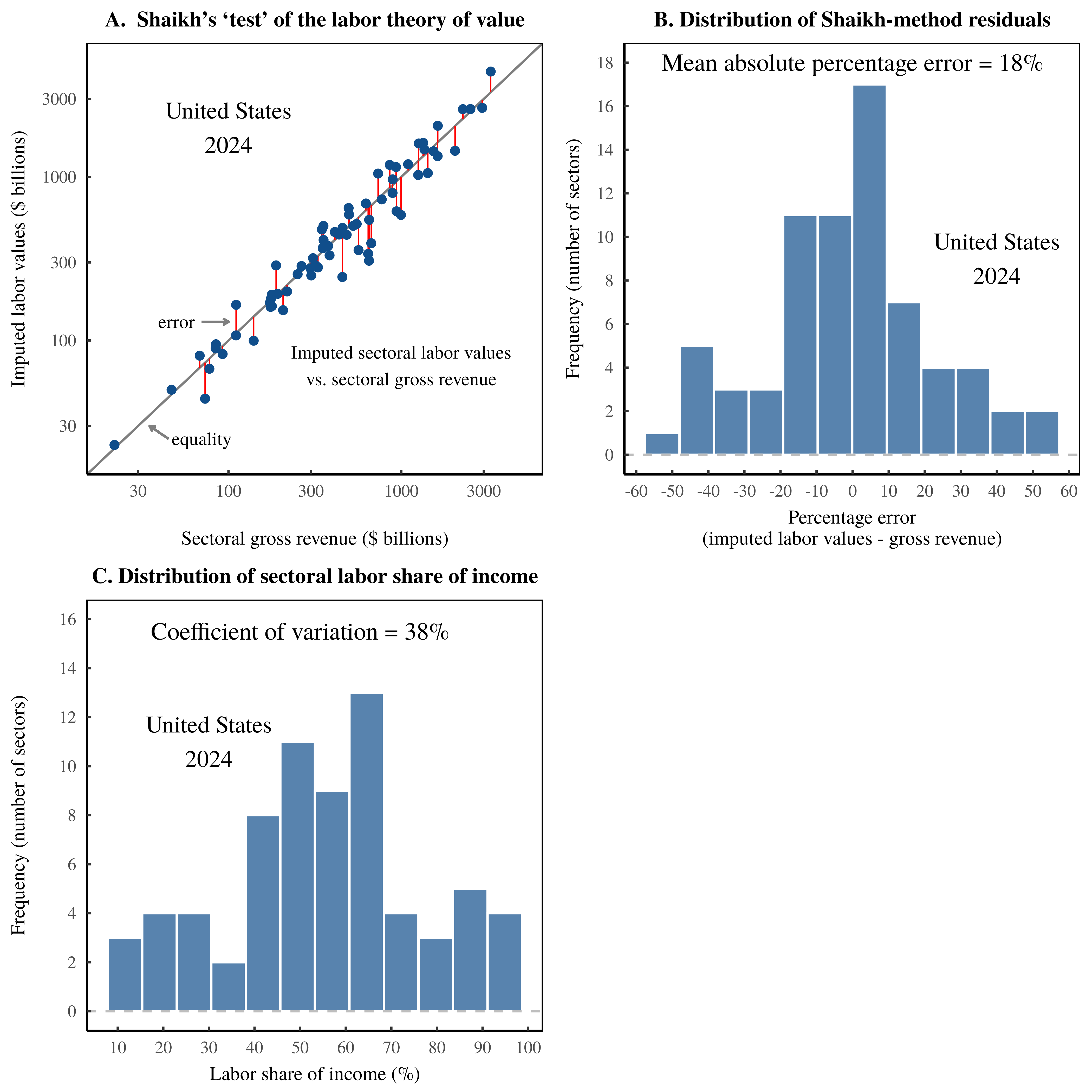Figure 8: The Shaikh method as noise transmutation.

This chart illustrates my hypothesis that Shaikh’s method for ‘testing’ the labor theory of value consists of an algorithm for transforming statistical noise. Using US data in 2024, Panel A shows the relation between imputed sectoral labor values and sectoral gross revenue. (Each point represents a sector.) The vertical red lines indicate the error in the Shaikh method — the portion of gross revenue that is unexplained by imputed labor values. The actual science of Shaikh’s method, I argue, lies in this noise. In Panel B, I have plotted the distribution of the Shaikh-method residuals. My contention is that this statistical noise is, in turn, a function of the cross-sector dispersion in the share of income, dispersion which I have visualized in Panel C. For the sources and methods behind these calculations, see the Appendix.

---

To test my noise hypothesis, I will implement Shaik’s method many times on different sets of data. But first, let’s define the required measurements. I will measure the spread of Shaikh-method residuals using the mean absolute percentage error between imputed labor values, \footnotesize v , and sectoral gross sales, \footnotesize g :

\text{shaikh-method error} = \text{mean} \left( \frac{ | v - g |}{g} \right )(50)

And I will measure the cross-sector spread of the labor share of income, \footnotesize \overline{L} , using the coefficient of variation:

\text{dispersion in} ~ \overline{L} = \frac{ \text{sd} ( \overline{L} ) }{ \text{mean} ( \overline{L} ) } (51)

To test my noise hypothesis, I head first to the United States, where I run Shaikh’s method on national accounting data from 1997 to 2024. Figure 9 shows the results. Here, each point shows the Shaikh-method results for a specific year of US data. The vertical axis shows the average error in the Shaikh method. And the horizontal axis shows the cross-sector dispersion in the labor share of income. Notice the connection between the two forms of statistical noise.

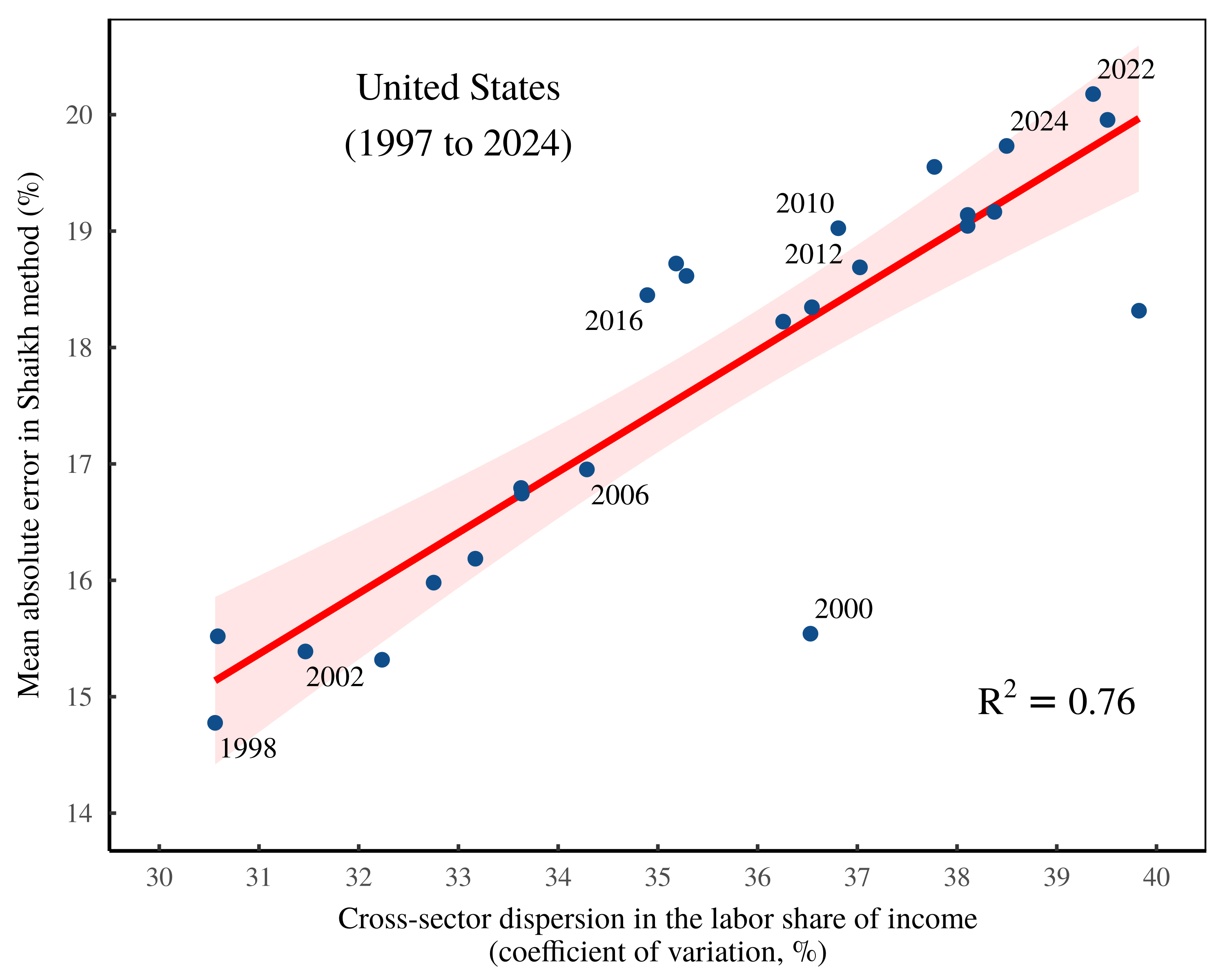Figure 9: Noise transmutation in the United States.

This chart shows the results of repeatedly implementing the Shaikh method on US national accounts data ranging over the years 1997 to 2024. Each point indicates an annual result. The vertical axis plots the statistical noise in the Shaikh method — the mean absolute percentage error between imputed labor values and sectoral gross revenue. The horizontal axis shows cross-sector dispersion in the labor share of income, as measured by the coefficient of variation. For the sources and methods behind this chart, see the Appendix.

---

If Shaikh’s algorithm offered a genuine measurement of the value created by labor, then the pattern in Figure 9 is baffling. Yes, Marx assumed that commodity prices would oscillate around their labor values. But why would this statistical noise be a function of the cross-sector dispersion in the labor share of income? I can think of no plausible reason.

Of course, we know that Shaikh’s algorithm does not measure labor values; rather, it imposes this metaphysical concept onto labor costs. And from there, the math leads to an awkward conclusion, which US data seems to verify. The Shaikh method takes noise in the labor share of income and transforms it into more muted noise between imputed labor values and sectoral gross revenue.

Widening the lens, I will now repeat this noise-measurement procedure across many more countries. To do that, I turn to OECD national accounting data, which covers 57 countries from the years 1995 to 2022. Using this data, I have implemented Shaikh’s method over 1500 times; each iteration compares the Shaikh-method residuals to cross-sector dispersion in the labor share of income.

Figure 10 shows the results of this analysis. First, note that the OECD data greatly expands the statistical breadth of the investigation. (For reference, the green box illustrates the range of US data plotted in Figure 9.) Second, note that the trend remains similar to the US pattern. Across these many observations, noise in the Shaikh method is explained largely by cross-sector dispersion in the labor share of income.

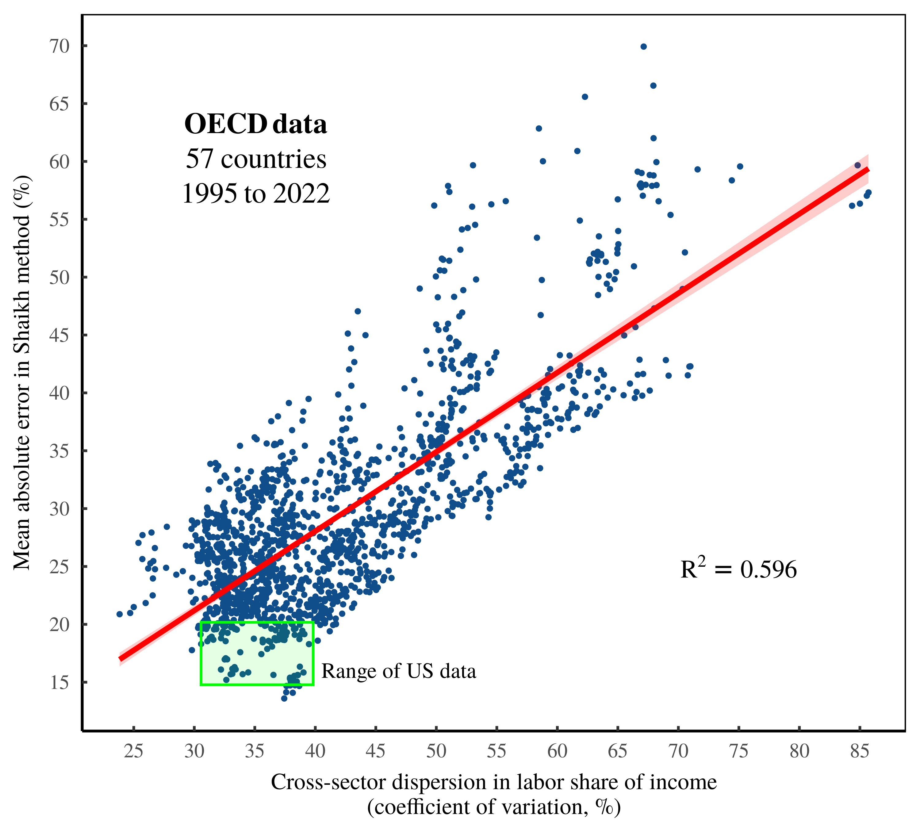Figure 10: Noise transmutation among OECD countries.

This chart shows the results of repeatedly implementing the Shaikh method on OECD national accounts data ranging over 57 countries from 1995 to 2022. Each point indicates a country-year result. The vertical axis plots the statistical noise in the Shaikh method — the mean absolute percentage error between imputed labor values and sectoral gross revenue. The horizontal axis shows cross-sector dispersion in the labor share of income, as measured by the coefficient of variation. For reference, the green square indicates the range of US data shown in Figure 9. For the sources and methods behind this chart, see the Appendix.

---

The US Rube-Goldberg model

Given the evidence in Figures 9 and 10, it seems clear that Shaikh’s ‘test’ of the labor theory of value amounts to an algorithm for transforming statistical noise. As a final demonstration of this principle, I now present the US ‘Rube-Goldberg model of noise transmutation’.

In this model, the entire apparatus of the US national accounts (including the calculation of the Leontief inverse matrix) serves as a machine for manipulating and transforming synthesized statistical noise. This noise consists of randomly generated data for the labor share of income — data designed to span the whole range of noise parameter space. And the Rube-Goldberg machine consists of the rest of Shaikh’s algorithm, fed real-world data from the United States.

Figure 11 shows the results of the Rube-Goldberg model. As expected, noise in the Shaikh method is driven largely by cross-sector dispersion in the labor share of income. But with the help of our synthesized labor income, we now see the full parameter space of our noise-transmutation algorithm. And just as predicted, when the labor share of income becomes uniform across sectors (meaning input noise collapses to zero), the Shaikh method produces an output with negligible statistical noise. In other words, it generates a beautifully circular ‘test’ of the labor theory of value.

(Note that the structure of the US empirical data prevents the Shaikh residuals from collapsing all the way to zero. In the Appendix, I show that this limit is largely a consequence of the data’s floating-point accuracy.)

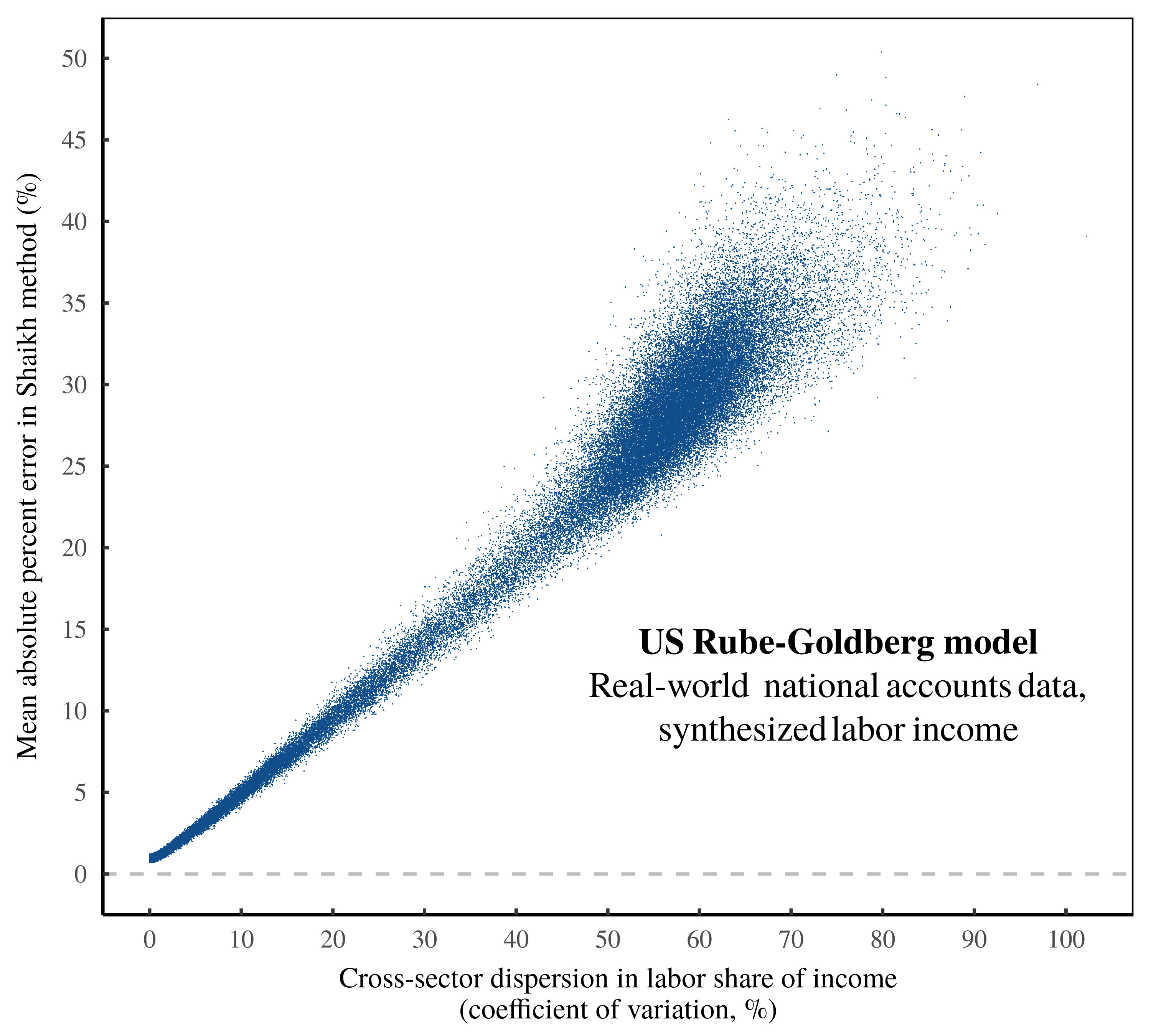Figure 11: The US Rube-Goldberg model of noise transmutation.

As a final demonstration that Shaikh’s ‘test’ of the labor theory of value is a form of noise transmutation, this chart shows the results of the US ‘Rube-Goldberg model’. In this model, the entire apparatus of the Shaikh method (including the US national accounting data) consists of an algorithm for manipulating synthesized noise in the labor share of income. This chart shows the results of implementing the Rube-Goldberg model 100,000 times. (Each point represents an iteration.) The vertical axis plots the statistical noise in the Shaikh method — the mean absolute percentage error between imputed labor values and sectoral gross revenue. The horizontal axis shows cross-sector dispersion in the labor share of income, as measured by the coefficient of variation. Note that as noise in the labor share of income collapses to zero, the error in the Shaikh method vanishes, indicating a perfectly circular ‘test’ of the labor theory of value. For the sources and methods behind this chart, see the Appendix.

---

The metaphysical kill switch

Humans, being emotional creatures, have great difficulty not interpreting evidence in a way that flatters our prior beliefs. Science, I would argue, is the only known solution to this problem. In science, the goal is to be explicit about the ways that an idea can be wrong — so explicit that if and when conflicting evidence turns up, the violation is obvious.

Metaphysics, in contrast, is a method for ensured belief-flattery. With metaphysics, we frame beliefs in a way that makes their ingredients unobservable, hence the belief can be maintained in the face of a wide range of evidence. All religions rely on this metaphysical trick. And sadly, a large portion of the social sciences play the same game.

Economics is a particularly egregious metaphysical offender, in large part because of the phenomenon it studies. Money. Money may not be the root of all evil, but it is the root of most misunderstandings in economics. The problem, put simply, is that money allows a simple quantification of a qualitative process that is bafflingly complex. And this qualitative process is, well, human society. To put it plainly, money is a clever numerical method for quantifying human social relations. The numerical output — a price — is crisp and clean. The qualitative input — human relations — is hopelessly messy.¹⁴

Faced with the quantitative crispness of prices, economists have historically been gripped by the urge to see an equally pristine number lying beneath the monetary surface. But when we search for this underlying quanta we never find it. Which is, of course, because the quanta is metaphysical; it is by definition unobservable. Undeterred, economists retreat to their imaginations, where they are free to impose their metaphysical quanta onto the thing that the quanta is supposed to explain: prices. With this metaphysical alchemy in hand, the stage is set for an endless parade of (pretend) tests of the metaphysics in question.

To be clear, the tragedy of this metaphysical thinking is not that it is wrong. After all, being wrong is a key part of science. No, metaphysical thinking is pernicious because it is a scientific kill switch. Evolutionary biology offers a good example. For centuries, humans unearthed fossils, but deemed this evidence an uninteresting quirk of ‘divine creation’. It was only when Darwin (1859) removed this religious metaphysics that the fossil evidence was taken seriously as a historical record of life on Earth.

Turning to political economy, monetary data is a rich source of evidence about human society, but one that can be misunderstood when metaphysical thinking gets involved. Amusingly, much of the misunderstanding comes from a failure to appreciate the rules of double-entry bookkeeping — rules which we have created.

A key feature of double-entry bookkeeping is that it defines relations between categories of value. These definitions, in turn, create what I call ‘bookkeeping correlations’. For example, if I earn more money, I will also tend to spend more money. Hence my income and expenses will correlate. Now, a big part of observational science involves finding correlations, because these relations offer clues about cause and effect. But in the case of bookkeeping relations, the correlation is uninteresting because the statistical noise is preordained — we can state its functional form before we even look at the data. So when it comes to bookkeeping relations, it is the noise, not the correlation, that is scientifically interesting.

The tragedy of metaphysics (including the Marxist variety) is that it distracts us from fascinating statistical noise that is driven by differences in income. The double tragedy is that heterodox thinkers like Anwar Shaikh have developed ingenious techniques for studying income differences, only to mistake these tools as a way to ‘test’ the labor theory of value — a theory which from the outset, has been untestable.¹⁵

Metaphysics aside, it is worth giving Shaikh credit for creating an algorithm that is legitimately useful. Indeed, when Shaikh’s method is restrained to its proper bookkeeping domain, it gives intriguing insights into the distribution of income. The question being asked is this: if I spend a dollar into a given sector, what portion of this money is eventually paid to workers? Shaikh’s method answers this question.

As an illustration, Figure 12 shows what happens when we use Shaikh’s method to calculate total labor costs across US sectors, measured as a share of gross revenue. The variation (the noise) in these values is fascinating. For example, in the petroleum sector, less than 30 cents on every dollar of revenue ends up getting paid to workers. Whereas for federal government enterprises, workers receive closer to 80 cents on every dollar of gross revenue.

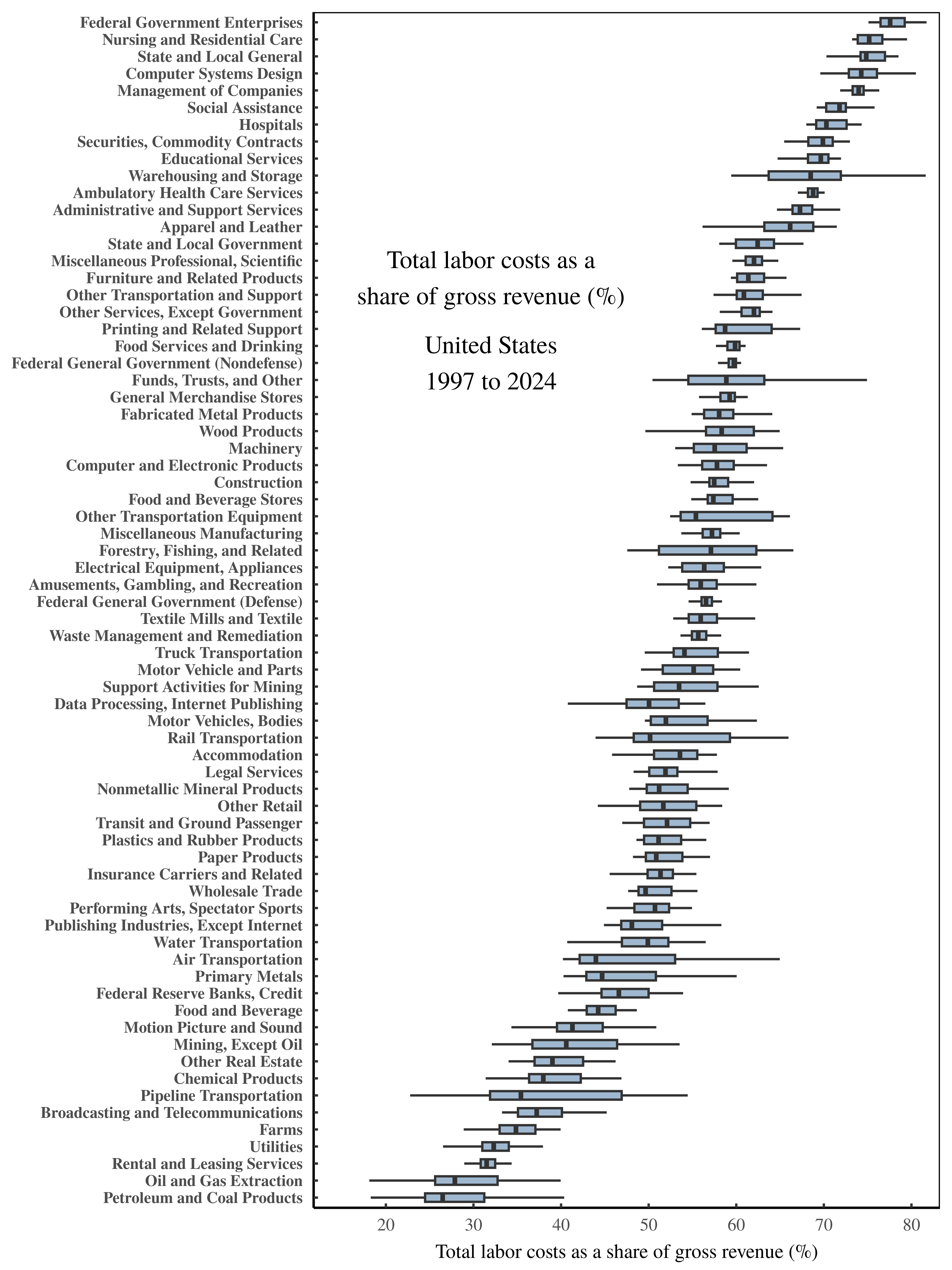Figure 12: Total labor costs as a share of gross revenue across US sectors.

This chart shows (what I see as) the scientific content of the Shaikh method. When Shaikh’s algorithm is stripped of its metaphysics and constrained to its proper domain of financial bookkeeping, it allows us to measure, for each sector, the portion of gross revenue that is eventually paid to workers at large. Here, I’ve calculated this labor portion across US sectors over the years 1997 to 2024. (Each boxplot shows the range of sectoral values over time.) Note that there is significant variation across sectors — variation which deserves to be explained. For the sources and methods behind this chart, see the Appendix.

When Shaikh’s method is presented in its proper bookkeeping domain, it immediately leads to more questions. How does the petroleum sector avoid sending money to workers? Why do government enterprises exhibit the opposite behavior? I’ll leave these questions unanswered, because my point is that the science lies in posing the questions in the first place.¹⁶

In contrast, the effect of metaphysics is to pre-emptively ‘answer’ questions before they have ever been posed. Why do fossils exist? In the context of religious metaphysics, the question is pointless because we already ‘know’ the answer: god did it. Likewise, in the context of Marxian metaphysics, it is pointless to ask why there is cross-sector variation in total labor costs as a share of gross revenue. We already know the answer: the variation is uninteresting ‘noise’ in a verification of the master’s work.

To conclude this study of Marxist metaphysics, it is always possible to impose onto bookkeeping relations quantities that are otherwise unobservable. For this reason, metaphysical alchemy will almost surely remain a reliable part of economists’ toolkit. But for those who lack the faith, know that when it comes to bookkeeping relations, the science lies in the noise.

Sources and methods

All the data and code used in this paper is available at the Open Science Framework: https://osf.io/czsju

Shaikh’s (untransmogrified) method for calculating total labor costs

Here I present the untransmogrified version of Shaikh’s analysis, by which I mean a version that removes the Marxian and Sraffian rhetorical transmutations, and leaves behind the straightforward manipulation of accounting categories. (Credit goes to Sabatino for doing most of the work untangling Shaikh’s algebra.)

In my view, the most straightforward presentation of Shaikh’s method is that it provides a way to calculate total (direct + indirect) labor costs as a share of sectoral gross revenue:

\boldsymbol{l_t} \oslash \boldsymbol{g} = ( \boldsymbol{l} \oslash \boldsymbol{g}) ~ \left( \boldsymbol{I} - \boldsymbol{A} \right)^{-1} (52)

Let me first clarify this notation. In Equation 52, bold lowercase symbols denote a vector, which consists of a list of values across sectors. Bold uppercase symbols denote a matrix, which consists of a table of values across sectors.

Next, Shaikh’s method makes use of both matrix mathematics, as well as element-wise operations on vectors. To distinguish these operations, I introduce the ‘ \footnotesize \oslash ’ to indicate element-wise division. For example, the operation \footnotesize \boldsymbol{l_t} \oslash \boldsymbol{g} denotes element-wise division of the vectors \footnotesize \boldsymbol{l_t} and \footnotesize \boldsymbol{g} :

\boldsymbol{l_t} \oslash \boldsymbol{g} = \begin{bmatrix} l_{t_1} / g_1 \\ l_{t_2} / g_2 \\ \vdots \\ l_{t_i} / g_i \\ \end{bmatrix} (53)

In contrast, when there are no symbols connecting adjacent variables, this operation denotes matrix multiplication.

Now to the various terms in Equation 52. As I see it, the natural output of Shaikh’s method is the vector \footnotesize \boldsymbol{l_t} \oslash \boldsymbol{g} . It consists of the total (direct + indirect) labor costs, \footnotesize l_t in each sector, reported per dollar of sectoral gross revenue, \footnotesize g . Perhaps the most useful interpretation of this value is that it is a statement about the distribution of income. If we spend $1 dollar into sector \footnotesize i , Shaikh’s method reports the portion of this money that is ultimately received by workers (across the entire society).

To calculate this labor portion, we start by calculating \footnotesize \boldsymbol{l} \oslash \boldsymbol{g} , which consists of direct labor costs, \footnotesize l , measured as a share of sectoral gross revenue, \footnotesize g , and reported across all sectors:

\boldsymbol{l} \oslash \boldsymbol{g} = \begin{bmatrix} l_1 / g_1 \\ l_2 / g_2 \\ \vdots \\ l_i / g_i \\ \end{bmatrix} (54)

To transform direct labor costs into total labor costs, we multiply the vector \footnotesize \boldsymbol{l} \oslash \boldsymbol{g} by the Leontief inverse matrix. This latter quantity consists of an algebraic method for tracking the full web of intersectoral transactions:

\text{Leontief inverse matrix} = ~ \left( \boldsymbol{I} - \boldsymbol{A} \right)^{-1} (55)

Turning to real-world data, there are several ways to acquire the Leontief inverse matrix. First, one can download the data directly from government statistical agencies. In the United States, this data is called the ‘Industry-by-Industry Total Requirements Table’, and is published by the Bureau of Economic Analysis. In the OECD database, the data is reported as the ‘Leontief inverse’.

Another option is to calculate the Leonfief inverse from the matrix \footnotesize \boldsymbol{A} , which is often called the ‘direct requirements table’. The matrix \footnotesize \boldsymbol{A} is similar to the example transaction table shown Figure 5, in the sense that each cell reports a transaction between two sectors, and columns track expenses spent by the same sector. The main difference, however, is that the direct requirements table normalizes columns by dividing each element by the sector’s gross revenue. As such, the elements of the direct requirements table track expenses spent from sector \footnotesize j to sector \footnotesize i , reported as a portion of sector \footnotesize j ’s gross revenue. In contrast to the Leontief inverse matrix, the direct requirements table is not often reported. However, it can be calculated from the ‘use table’ and the ‘make table’, using methods described below.

Back to Shaikh’s method. Once we have calculated total labor costs as a share of gross revenue, \footnotesize \boldsymbol{l_t} \oslash \boldsymbol{g} , we can extract the dollar value of these labor costs by multiply each element by sectoral gross revenue:

\boldsymbol{l_t} = ( \boldsymbol{l_t} \oslash \boldsymbol{g} ) \circ \boldsymbol{g} (56)

Here, the symbol ‘ \footnotesize \circ ’ denotes element-wise multiplication.

Putting everything together, the total labor costs plotted in Figure 3 are calculated using the following equation:

\boldsymbol{ l_t } = \left[ \left( \boldsymbol{l} \oslash \boldsymbol{g} \right) \left( \boldsymbol{I} - \boldsymbol{A} \right)^{-1} \right] \circ \boldsymbol{g} (57)

The nice thing about this algebraic operation is that it is ambivalent about the data it is fed. In other words, if we wish to measure the total (direct + indirect) money flowing to capitalists — as plotted in Figure 4 — we simply replace the labor cost term, \footnotesize l , with the capitalist income term \footnotesize k :

\boldsymbol{ k_t } = \left[ \left( \boldsymbol{k} \oslash \boldsymbol{g} \right) \left( \boldsymbol{I} - \boldsymbol{A} \right)^{-1} \right] \circ \boldsymbol{g} (58)

Now to Shaikh’s metaphysical alchemy. In Shaikh’s jargon, the term \footnotesize \boldsymbol{l} \oslash \boldsymbol{g} represents ‘skill-adjusted direct labor values per unit of output’. Similarly, the term \footnotesize \boldsymbol{l_t} \oslash \boldsymbol{g} represents ‘skill-adjusted total labor values per unit of output’. Finally, the term \footnotesize \boldsymbol{l_t} represents ‘total labor values’, which in Shaikh’s mind, are denoted in units of labor time. As such, this labor-time quantity must be transformed into monetary prices using the ‘monetary expression of labor time’, \footnotesize \mu . Shaikh then finishes the alchemy by calling his completed calculation ‘direct prices’, even though the imputed quantity says nothing about actual commodity prices. (He also rebrands sectoral gross revenue as ‘market prices’.)

Cutting through the alchemy, Shaikh’s imputation of the value produced by labor, which I will call \footnotesize \boldsymbol{v} , consists of a normalized version of total labor costs, \footnotesize \boldsymbol{l_t} :

\boldsymbol{v} = \mu \cdot \boldsymbol{l_t} (59)

Here, the normalization constant, \footnotesize \mu , ensures that total labor costs sum to total gross revenue across all sectors:

\sum \mu \cdot \boldsymbol{l_t} = \sum \boldsymbol{g} (60)

Backing out of this transmogrification, the scientifically useful part of Shaikh’s calculation is the quantity \footnotesize \boldsymbol{l_t} \oslash \boldsymbol{g} — the vector of total labor costs as a share of sectoral gross sales. It is this quantity which I have plotted in Figure 12. Its variation across sectors is fascinating, and deserves an explanation.

In contrast, Shaikh’s metaphysical alchemy reframes the cross-sector variation in \footnotesize \boldsymbol{l_t} \oslash \boldsymbol{g} as statistical noise — noise that slightly disturbs the otherwise pure autocorrelation between sectoral gross revenue and itself. To summarize, Shaikh’s method demonstrates how a clever (and useful) bookkeeping calculation can be corrupted by metaphysical nonsense.

Deriving the direct requirements table

As outlined by Sabatino, we can derive the direct requirements table, \footnotesize \boldsymbol{A} , as follows:

\boldsymbol{A} = ( \boldsymbol{V} ~ \widehat{\boldsymbol{q~} }^{-1} ) ( \boldsymbol{U} ~ \widehat{\boldsymbol{g~} }^{-1} ) (61)

Here, \footnotesize \boldsymbol{V} denotes the ‘Industry-by-Commodity Make Table’, a matrix that tracks sectoral gross revenue as a function of the ‘commodity’ being sold. Similarly, \footnotesize \boldsymbol{U} denotes the ‘Commodity-by-Industry Use Table’, a matrix that tracks sectoral purchases by the ‘commodity’ being bought. Note that in these tables, the term ‘commodity’ is a transmogrified variation of the term ‘sector’ — a variation in which statistical agencies attempt to decompose the revenue stream within firms.

The backstory is that the national accounts categorize transactions using firm boundaries, meaning they place a firm into a ‘sector’ based on its primary revenue stream. However, this method leads to counterintuitive outcomes. For example, a firm that earns most of its revenue from farming would have its non-farm revenue placed in the ‘farm’ sector. To ‘correct’ this problem, government statisticians introduce the ‘commodity view’ of sectors, in which they seek to decompose firm revenue (and expenses) based on their perceived form.

From this scheme comes two views for quantifying gross revenue. There is the ‘industry’ view of gross revenue, \footnotesize g , which categorizes transactions into sectors based on each firm’s main revenue source. Then there is the ‘commodity’ view of gross revenue, \footnotesize q , which ignores firm boundaries, and categorizes transactions based on their perceived form.

Importantly, the vectors \footnotesize \boldsymbol{q} and \footnotesize \boldsymbol{g} are themselves functions of the make table, \footnotesize \boldsymbol{V} :

\boldsymbol{q} = \boldsymbol{i} ~ \boldsymbol{V} (62)

\boldsymbol{g} = \boldsymbol{V} ~ \boldsymbol{i} (63)

Here, \footnotesize \boldsymbol{i} denotes a column vector filled with ones. The matrix operation \footnotesize \boldsymbol{i} ~ \boldsymbol{V} serves to take the column sums of \footnotesize \boldsymbol{V} . Likewise, the matrix operation \footnotesize \boldsymbol{V} ~ \boldsymbol{i} serves to take the row sums of \footnotesize \boldsymbol{V} .

Returning to Equation 61, the ‘ \footnotesize \widehat{~~~~} ’ symbol denotes placing a vector along the diagonal of zero-matrix, as follows:

\widehat{\boldsymbol{g}} = \begin{bmatrix} g_1 & 0 & \ldots & 0 \\ 0 & g_2 & \ldots & 0 \\ \vdots & \vdots & \ddots & \vdots \\ 0 & 0 & 0 & g_i \end{bmatrix} (64)

US data

All US data is from the Bureau of Economic Analysis (BEA), as follows:

• Employment by sector (Figure 1) is from Table 6.5D, Full-Time Equivalent Employees by Industry.

• Value added by sector (Figures 1 and 2) is from BEA interactive data, ‘value added by industry’ (which mysteriously comes without a table number).

• The ‘Shaikh method’ (Figures 3, 4, 7B, 8, 9, 11, 12). I bulk downloaded historical input-output data from https://apps.bea.gov/industry/release/zip/MAKE-USE-IMPORTS%20(AFTER%20REDEFINITIONS).zip.

  Specifically, I used the spreadsheet IOUse Before Redefinitions PRO Summary to define the use table, \footnotesize \boldsymbol{U} , and the spreadsheet IOMake Before Redefinitions PRO Summary to define the make table, \footnotesize \boldsymbol{V} . Data for the US Shaikh method is derived as follows:

1. In the use table, \footnotesize \boldsymbol{U} , I exclude scrap and imports, and include only intermediate purchases. (That is, I exclude the ‘final demand’ portion of the use table spreadsheet, which is not relevant to the Shaikh method).

2. I calculate the vector \footnotesize \boldsymbol{q} (which in input-output jargon is called ‘commodity gross output’), by taking the column sums of the make table, \footnotesize \boldsymbol{V} (Equation 62).

3. I calculate the vector \footnotesize \boldsymbol{g} (which in input-output jargon is called ‘industry gross output’), by taking the row sums of the make table, \footnotesize \boldsymbol{V} (Equation 63).

4. I use the ‘compensation of employees’ to measure direct labor costs, \footnotesize \boldsymbol{l} . (This data is contained in the summary rows of the use table spreadsheet.)

5. I use Equation 61 to calculate the direct requirements table, \footnotesize \boldsymbol{A} .

6. I use Equation 57 to calculate total (direct + indirect) labor costs, \footnotesize \boldsymbol{l_t} .

7. Direct pretax capitalist income, \footnotesize \boldsymbol{k} consists of the sum of ‘gross operating surplus’ and ‘taxes on production’, which are both found in the summary rows of the use table spreadsheet.

8. I use Equation 58 to calculate total (direct + indirect) pretax capitalist income, \footnotesize \boldsymbol{k_t} .

9. Sector value added, \footnotesize \boldsymbol{y} , comes from the summary rows of the use table spreadsheet.

10. The labor share of income is \footnotesize \boldsymbol{L} = \boldsymbol{l} / \boldsymbol{y} , the ratio of labor costs \footnotesize \boldsymbol{l} to value added \footnotesize \boldsymbol{y} .

11. Shaikh’s imputed labor values, which I call \footnotesize \boldsymbol{v} , consist of normalized total labor costs, \footnotesize \boldsymbol{l_t} , calculated using Equation 59 and Equation 60. Note that the normalization ensures that imputed labor values sum to total gross revenue across all sectors. The effect of this normalization is to center the Shaikh residuals (the difference between \footnotesize \boldsymbol{g} and \footnotesize \boldsymbol{v} ) around zero.

12. Once the Shaikh-method calculation is complete, I exclude results for the ‘Housing’ sector, which are contaminated by imputations for the (non-existent) rent that house owners pay to themselves.

    Note that in his original analysis, Shaikh includes the ‘Housing’ sector, but removes the owner-occupied imputations. In her replication of Shaikh’s work, Sabatino also undoes these imputations. But for my purposes here, I find it simpler to just exclude the ‘Housing’ sector from the results.

13. I calculate cross-sector dispersion in the labor share of income using the coefficient of variation of \footnotesize \boldsymbol{L} — the standard deviation divided by the mean:

\text{dispersion} (\boldsymbol{L} ) = \frac{ \text{sd}( \boldsymbol{L} ) } { \text{mean} ( \boldsymbol{ L } ) } (65)

14. I calculate the average residuals in Shaikh’s method using the mean absolute error:

    \text{error} ( \boldsymbol{v} ) = \text{mean} \left( ~ | \boldsymbol{v} - \boldsymbol{g}| \oslash \boldsymbol{g} \right) (66)

15. In my analysis in Figure 9, I have excluded the years 2008, 2018, and 2018. That’s because in these years, dispersion in the cross-sector labor share of income mysteriously jumps — a likely sign of data problems. See Figure 13 for a visualization of these outliers.

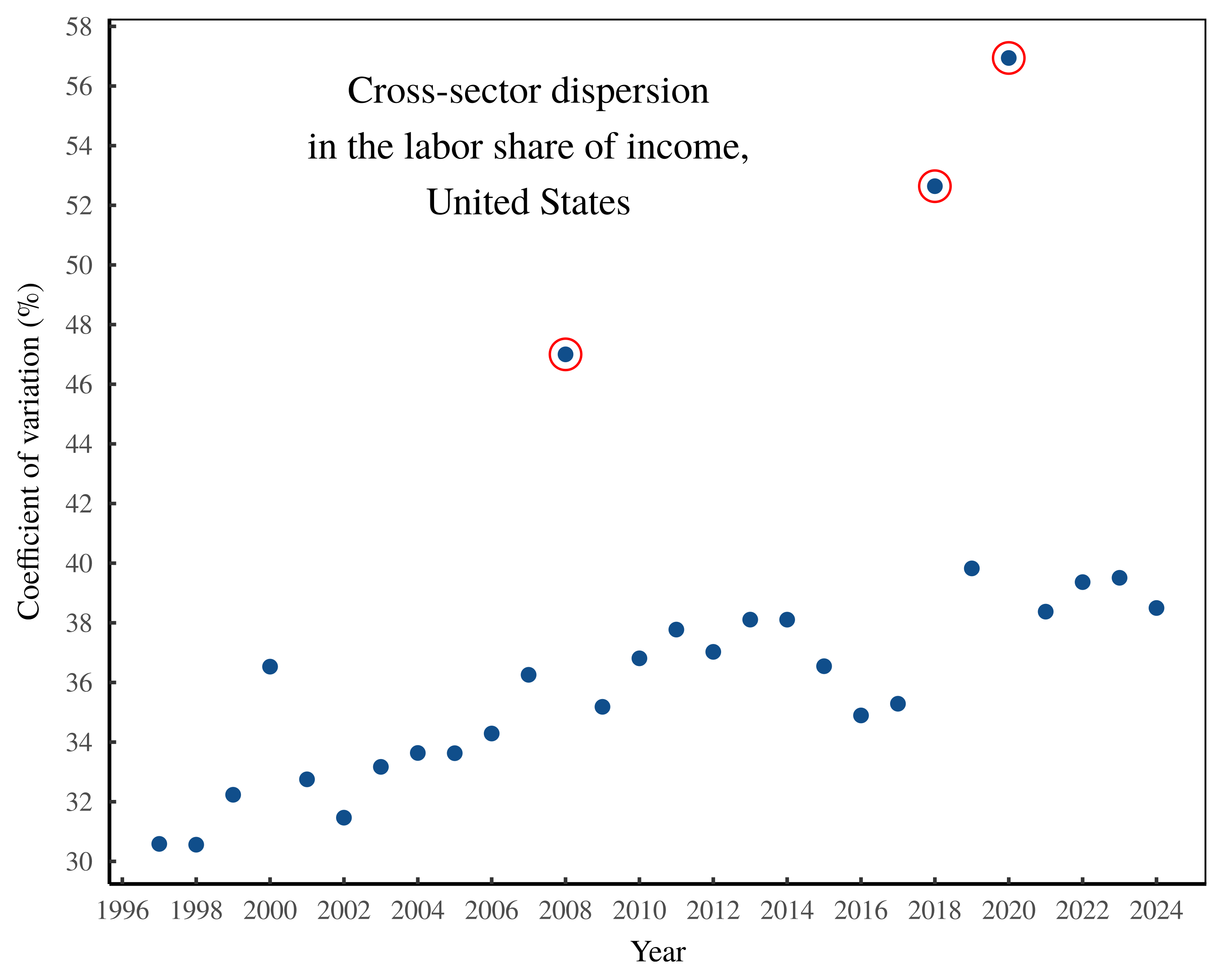Figure 13: Cross-sectoral dispersion in the US labor share of income.

When calculated from input-output tables, cross-sector dispersion in the US labor share of income has tended to rise with time. There are, however, three odd outliers, illustrated here with red circles. I have excluded these observations from the analysis in Figure 9.

---

US Rube-Goldberg model

The idea behind the US Rube-Goldberg model (Figure 11) is that the apparatus of Shaikh’s method can be treated as a complicated tool for generating statistical noise. Shaikh’s method takes as input, noise in the labor share of income, and returns as output, noise between imputed labor values and sectoral gross revenue.

To demonstrate this interpretation of Shaikh’s method, the US Rube-Goldberg model is essentially a function for taking real-world US input-output data and using it to transform synthesized labor costs, \footnotesize \boldsymbol{l_s} , into counterfactual imputed labor values, \footnotesize \boldsymbol{v_c} . The math looks like this:

\boldsymbol{ v_c } = \left[ \left( \boldsymbol{l_s} \oslash \boldsymbol{g_{e_i}} \right) \left( \boldsymbol{I} - \boldsymbol{ A_{e_i}} \right)^{-1} \right] \circ \boldsymbol{g_{e_i}} ~ \mu (67)

In Equation 67, the subscript \footnotesize e_i indicates the use of US empirical data in year \footnotesize i . (This empirical data is calculated using methods documented in the US data section. Note that the scalar \footnotesize \mu is a normalization constant which ensures that \footnotesize \sum \boldsymbol{ v_c } = \sum \boldsymbol{ g_{e_i} } .)

The steps for the Rube-Goldberg model are as follows:

1. I sample a year, \footnotesize i , from the range of US data, which runs from 1997 to 2024.

2. With this year selected, I calculate the empirical values for sectoral gross revenue, \footnotesize \boldsymbol{ g_{e_i}} , and the direct requirements table, \footnotesize \boldsymbol{ A_{e_i} } , using the methods discussed in the US data section.

3. Next, I synthesize values for sectoral direct labor costs, \footnotesize \boldsymbol{l_s} . The goal is to have these labor costs be a random portion of real-world value added, \footnotesize \boldsymbol{y_{e_i}} — a portion that can vary from 0% to 100%. To synthesize direct labor costs, I first sample random numbers from a truncated normal distribution. Let \footnotesize \boldsymbol{r} be a vector of random numbers sampled from a truncated normal distribution with a lower bound of 0, an upper bound of 1, and parameters \footnotesize \mu_r and \footnotesize \sigma_r :

   \boldsymbol{r} \sim \mathbb{N}(\mu_r, \sigma_r), ~ 0 \leq r \leq 1 (68)

   The vector of synthesized labor costs, \footnotesize \boldsymbol{l_s} , is then the element-wise product of \footnotesize \boldsymbol{r} and \footnotesize \boldsymbol{y_{e_i}} :

   \boldsymbol{l_s} = \boldsymbol{r} \circ \boldsymbol{y_{e_i}}(69)

4. To explore the parameter space of Shaikh’s method, I run the Rube-Goldberg model many times. Each iteration uses a different (randomly sampled) year for the US empirical data. Additionally, in each iteration, the parameters \footnotesize \mu_r and \footnotesize \sigma_r vary randomly in order to simulate differing degrees of dispersion in the labor share of income. Of course, the synthesized labor share of income, \footnotesize \boldsymbol{L_s} , is just the vector of random numbers, \footnotesize \boldsymbol{r} :

   \displaystyle \boldsymbol{ L_s} = \boldsymbol{ l_s} \oslash \boldsymbol{ y_{e_i} } = r

5. I measure dispersion in the synthesized labor share of income using Equation 65.

6. I measure the mean absolute error in Shaikh’s method using Equation 66.

Deviation from the smooth transaction approximation

One of the interesting things we can do with the US Rube-Goldberg model is to measure the accuracy of our preordained noise function:

\sigma \approx l_g + \frac{ L - l_g }{L} \cdot \overline{L} (70)

Recall that I derived this function by using the smooth-transaction approximation, which assumes that indirect labor costs are a function of the average labor share of income. To the degree that this approximation breaks down, the full-scale Shaikh method will create noise that is not predicted by Equation 70.

To measure this deviation, we need to measure the spread of our noise function using the mean absolute percentage error (which is how we measured noise in the Shaikh method). Let the ‘error’ in our noise function be the deviation from the mean:

\text{error}(\sigma) = \text{mean} \left( \frac{ | \sigma - \overline{\sigma} | }{ \overline{\sigma} } \right)(71)

And to reiterate, the error in the full-scale method is the deviation between imputed labor values, \footnotesize v and sectoral gross revenue, \footnotesize g :

\text{error}(v) = \text{mean} \left( \frac{ | v - g | }{ g } \right)(72)

If we subtract these two forms of error, we can measure the degree to which the full-scale Shaikh method deviates from the smooth transaction limit:

\text{Deviation from STA} = \text{error} (v) - \text{error}(\sigma) (73)

Figure 14 plots this deviation in the Rube-Goldberg model. Unsurprisingly, the deviation depends on cross-sector dispersion in the labor share of income. When the labor share of income is quite uniform across sectors, our preordained noise function accurately predicts the noise in the full-scale Shaikh method. But when the labor share of income varies greatly across sectors, the preordained noise function poorly predicts the noise generated by the full-scale Shaikh method.

The irony here is that the full-scale Shaikh method seems to be most indispensable in situations when it will generate maximum noise between imputed labor values and sectoral gross revenue. Which is to say that the method is scientifically useful in situations where it appears to falsify the labor theory of value.

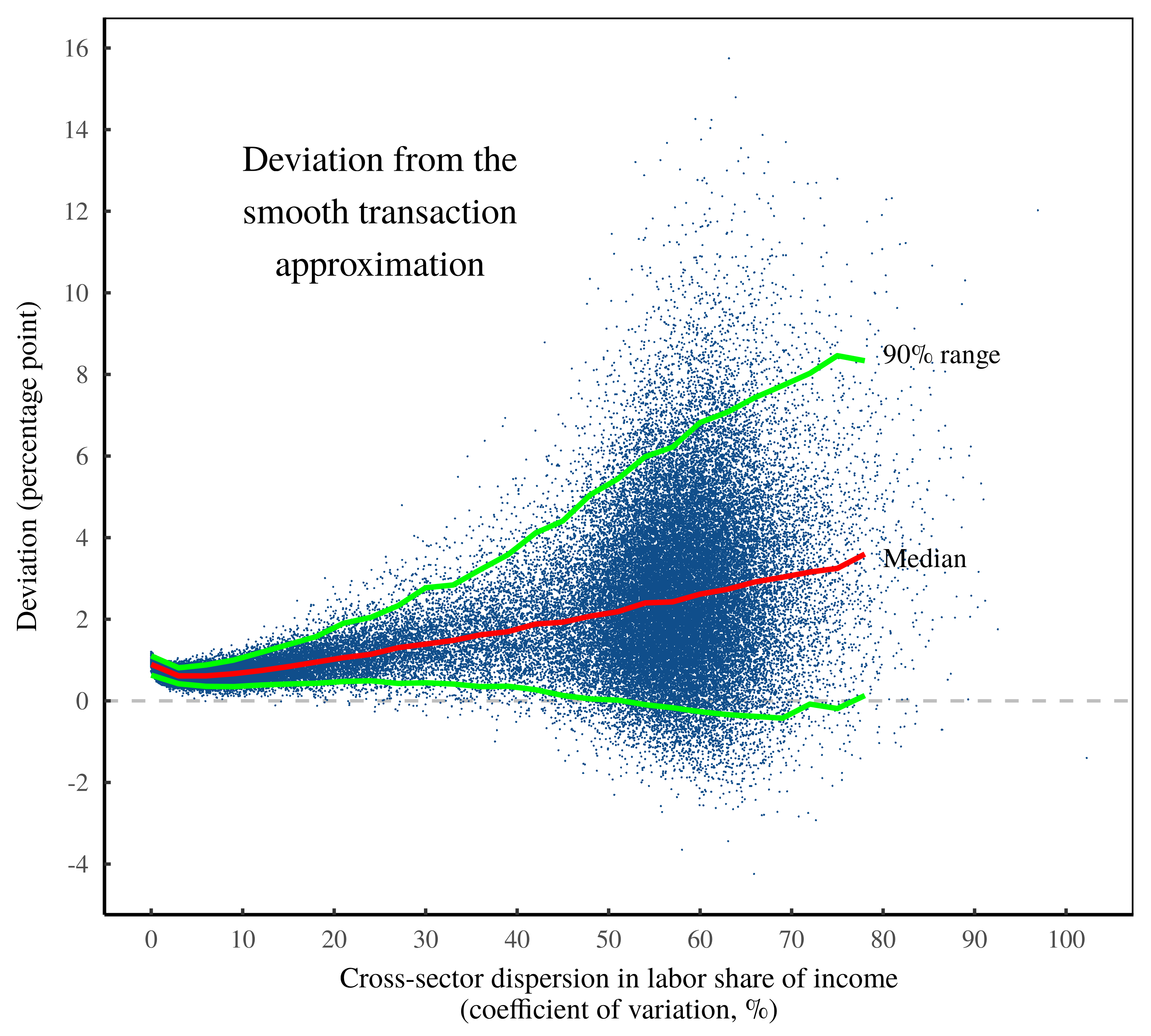Figure 14: Deviation from the smooth transaction approximation in the US Rube-Goldberg model.

Using the US Rube-Goldberg model, this chart measures how well the smooth-transaction approximation predicts the statistical noise in the full-scale Shaikh method. (Each point represents an iteration of the model.) Here, the vertical axis shows the difference between the two approaches — the noise generated by the full-scale Shaikh method minus the noise generated by the smooth-transaction approximation. (Both forms of noise are measured using the mean absolute percentage error.) In general, the full-scale Shaikh method generates slightly more statistical noise than the smooth-transaction approximation. But just how much more noise turns out to be a function of the cross-sector dispersion in the labor share of income (horizontal axis). To illustrate the trend, the red line shows the median of the data points. The green lines show the 90% range.

---

OECD input-output data

OECD input-output data is available at: https://www.oecd.org/en/data/datasets/input-output-tables.html

Figure 10 uses data from the OECD 2025 release, which includes data for 58 countries covering the years 1995 to 2022. (In Figure 10, I have excluded data for the Republic of Congo, which lies far outside the range for all other countries.) The steps for the OECD calculations are as follows:

1. Direct labor costs, \footnotesize \boldsymbol{l} , come from the VAcomponents.csv, using series LABR.

2. Domestic gross revenue, \footnotesize \boldsymbol{g} , comes from tables NATIODOMIMP, using series OUTPUT.

3. Domestic value added, \footnotesize \boldsymbol{y} , comes from tables NATIODOMIMP, using series VALU.

4. The labor share of income is the ratio of direct labor costs to value added: \footnotesize \boldsymbol{L} = \boldsymbol{l} / \boldsymbol{g} .

5. The domestic Leontief inverse matrix, \footnotesize ( \boldsymbol{I} - \boldsymbol{A} ) ^{-1} , comes from the tables NATLEONTFD.

6. For each country-year observation, I calculate total (direct + indirect) labor costs using Equation 57.

7. I calculate imputed labor values using Equation 59.

8. I calculate dispersion in the labor share of income using Equation 65.

9. I calculate the mean absolute error in the Shaikh method using Equation 66

A minimal stochastic model of Shaikh’s method

Here is how I create the model used in Figure 7. First, I let \footnotesize n be the number of sectors in the model, a value which can be any whole number. I then define the vector of sectoral gross revenue, \footnotesize \boldsymbol{g} , which consists of \footnotesize n random numbers sampled from a lognormal distribution:

\boldsymbol{g} \sim \ln \mathcal{N} ( \mu_g, \sigma_g ) (74)

Next, I model sectoral value added as follows. First, I sample a vector of \footnotesize n random numbers from a uniform distribution, ranging between zero and one:

\boldsymbol{r_1} \sim \mathcal{U} ( 0, 1 ) (75)

Then I define sectoral value added, \footnotesize \boldsymbol{y} to be the element-wise product of \footnotesize \boldsymbol{r} and \footnotesize \boldsymbol{g} :

\boldsymbol{y} = \boldsymbol{r} \circ \boldsymbol{g} (76)

The idea here is that value added can be any (positive) portion of sectoral gross revenue. Once I’ve created \footnotesize \boldsymbol{y} , I define intermediate expenses, \footnotesize \boldsymbol{e} , as the difference between gross revenue and value added:

\boldsymbol{e} = \boldsymbol{g} - \boldsymbol{y} (77)

Next, I generate the direct requirements table, \footnotesize \boldsymbol{A} , through the following steps. First, I fill the matrix \footnotesize \boldsymbol{A_1} with \footnotesize n^2 random numbers from a lognormal distribution:

\boldsymbol{A_1} \sim \ln \mathcal{N} ( \mu_A, \sigma_A ) (78)

Next, I normalize the matrix \footnotesize \boldsymbol{A_1} such that its columns sum to the vector of intermediate expenses, \footnotesize \boldsymbol{e} , as required by national accounting identities. In terms of matrix algebra (which I find opaque compared to R code), I define the normalized matrix \footnotesize \boldsymbol{A_2} such that:

\boldsymbol{A_2} = \boldsymbol{A_1} \left( \widehat{ \boldsymbol{i} \boldsymbol{A_1}} \right) ^{-1} ~ \widehat{ \boldsymbol{e~} } (79)

Breaking down the math, the operation \footnotesize \boldsymbol{i} \boldsymbol{A_1} denotes taking the column sums of \footnotesize \boldsymbol{A_1} . The operation \footnotesize \widehat{ \boldsymbol{i} \boldsymbol{A_1}} denotes putting these column sums along the diagonal of a matrix where all other values are zeros. The exponent \footnotesize -1 then indicates taking the inverse of this diagonal matrix, which in this special case, is equivalent to taking the reciprocal of each element. When we then matrix multiply \footnotesize \boldsymbol{A_1} by \footnotesize \left( \widehat{ \boldsymbol{i} \boldsymbol{A_1}} \right) ^{-1} , we normalize \footnotesize \boldsymbol{A_1} such that each column sums to one. Finally, multiplying by \footnotesize \widehat{ \boldsymbol{e~} } renormalizes our matrix so that the columns some to the elements of \footnotesize \boldsymbol{e} .

With our normalized matrix \footnotesize \boldsymbol{A_2} , we can then define the direct requirement matrix \footnotesize \boldsymbol{A} . The idea is that \footnotesize \boldsymbol{A} reports each sector’s intermediate expenses as a portion of its gross revenue. To define \footnotesize \boldsymbol{A} , we take the matrix \footnotesize \boldsymbol{A_2} and divide each column by the corresponding element for sectoral gross revenue. In terms of matrix math, that operation looks like this:

\boldsymbol{A} = \boldsymbol{A_2} ~ \widehat{\boldsymbol{g~} }^{-1} (80)

Next, I simulate the sectoral labor share of income, \footnotesize L , by sampling random numbers from a truncated normal distribution, with bounds of zero and one:

\boldsymbol{L} \sim \mathbb{N}(\mu_L, \sigma_L), ~ 0 \leq r \leq 1 (81)

I then calculate direct sectoral labor income, \footnotesize \boldsymbol{l} , by element-wise multiplying the labor share of income by value added, \footnotesize \boldsymbol{y} :

\boldsymbol{l} = \boldsymbol{L} \circ \boldsymbol{y}(82)

With this simulated data, I then use Equation 57 to calculate total (direct + indirect) labor costs.

The floating point limit to perfect autocorrelation in the Shaikh method

Looking closely at the behavior of the US Rube-Goldberg model in Figure 11, we can see that the error in the Shaikh method does not collapse all the way to zero in the limit that the labor share of income is perfectly uniform across sectors. The reason likely owes to the floating point accuracy of the input-output data published by the BEA.

To illustrate the effect of data accuracy, I will use the model outlined in the previous section, with two slight differences. First, I make the labor share of income, \footnotesize \boldsymbol{L} , perfectly uniform across sectors. The expectation, therefore, is that Shaikh’s method will return zero error between sectoral gross revenue and imputed labor values. Second, after calculating the direct requirements matrix, \footnotesize \boldsymbol{A} , I limit the accuracy of its values to a predefined number of significant digits. Then I implement Shaikh’s method on this accuracy-limited data.

As one might expect, the accuracy of the input data directly affects the accuracy of the Shaikh-method output. Figure 15 shows the effect. Here the horizontal axis shows the accuracy limit within the direct requirements table, measured by the number of significant digits. The vertical axis shows the corresponding error in Shaikh’s method.

In this model, the expected theoretical error is zero. However, imperfect data intervenes to mute this theoretical result. For example, when input data is limited to one significant digit, it creates generic error in the Shaikh method of about 1%. But as the input data becomes more accurate, the error in Shaikh’s method plunges exponentially towards zero. In this example, the limits of floating-point computation intervene when the data accuracy reaches 16 significant digits. Afterwards, error in the Shaikh method plateaus, simply because the computation itself cannot get more accurate. The lesson here is that we can numerically verify the circular limit to Shaikh’s method to whatever precision our computation allows.

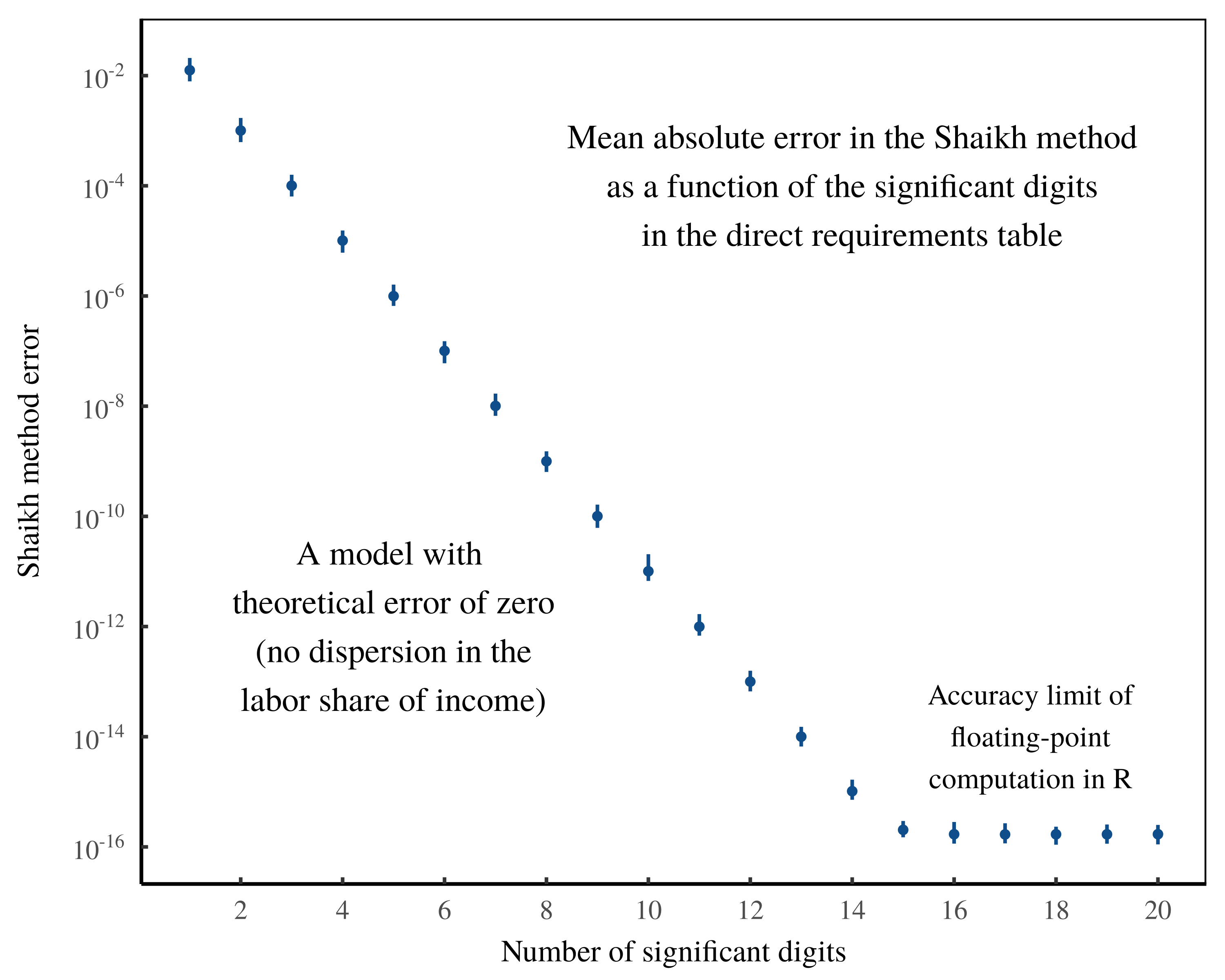Figure 15: The floating point limit to perfect autocorrelation in the Shaikh method. In numerical terms, the degree to which Shaikh’s method collapses to a tautology is limited by the float-point accuracy of the input data. This chart illustrates the pattern when Shaikh’s algorithm is implemented on simulated data that is designed to have zero theoretical error. (In this model, the labor share of income is constant across sectors.) Here, the horizontal axis shows the number of significant digits retained in the ‘direct requirements table’ — the table that is used to calculate total labor costs (and therefore, to impute ‘labor values’). The vertical axis shows the resulting error in the Shaikh method — the mean absolute error between imputed labor values and sectoral gross revenue. The points and error bars indicate the model mean and range over several thousand iterations. The Shaikh-method error decreases as the input data becomes more accurate. Note, however, that the error plateaus at around 15 significant digits, corresponding to the accuracy limit of floating point computation in R.

Notes

Blair Fix is a political economist based in Edmonton. He is the author of the book Rethinking Economic Growth Theory from a Biophysical Perspective. He blogs about his research at economicsfromthetopdown.com. Email: blairfix@fastmail.com

References

Cockshott, P., Cottrell, A., & Michaelson, G. (1995). Testing Marx: Some new results from UK data. Capital & Class, 19(1), 103–130.
Darwin, C. (1859). On the origin of species. London: John Murray.
Eatwell, J. (1975). Mr. Sraffa’s standard commodity and the rate of exploitation. The Quarterly Journal of Economics, 89(4), 543–555.
Fix, B. (2018). The trouble with human capital theory. Real-World Economics Review, 86, 15–32.
Leontief, W. (1953). Studies in the structure of the American economy: Theoretical and empirical explorations in input-output analysis. Oxford University Press.
Marx, K. (1867). Capital, volume I. Harmondsworth: Penguin/New Left Review.
Nitzan, J., & Bichler, S. (2009). Capital as power: A study of order and creorder. New York: Routledge.
Ochoa, E. M. (1989). Values, prices, and wage-profit curves in the US economy. Cambridge Journal of Economics, 13(3), 413–429.
Popper, K. (1959). The logic of scientific discovery. New York: Hutchinson & Co.
Ricardo, D. (1817). Principles of political economy and taxation. London: G. Bell; Sons.
Robinson, J. (1962). Economic philosophy. Chicago: Aldine Pub. Co.
Sabatino, I. K. (2026). Humbug labor values. Review of Capital as Power, 2(3), 1–52.
Shaikh, A. (1974). Laws of production and laws of algebra: The humbug production function. The Review of Economics and Statistics, 56(1), 115–120.
Shaikh, A. (1984). The transformation from Marx to sraffa. Ricardo, Marx, Sraffa, 43–84.
Shaikh, A. (1998). The empirical strength of the labour theory of value. In Marxian economics: A reappraisal: Volume 2: Essays on volume III of capital profit, prices and dynamics (pp. 225–251). Springer.
Shaikh, A. (2016). Capitalism: Competition, conflict, crises. Oxford University Press.
Smith, A. (1776). An inquiry into the nature and causes of the wealth of nations. Edinburgh: A.; C. Black.
Sraffa, P. (1960). Production of commodities by means of commodities: Prelude to a critique of economic theory. London: Cambridge University Press.
Stanovich, K. E., West, R. F., & Toplak, M. E. (2013). Myside bias, rational thinking, and intelligence. Current Directions in Psychological Science, 22(4), 259–264.
Tsoulfidis, L. (2021). Ricardo’s labor theory of value is alive and well in contemporary capitalism. World Review of Political Economy, 12(4), 493–518.