Productivity and Income … Again

Productivity and Income … Again

December 17, 2020

Originally published on Economics from the Top Down

Blair Fix

Today I’m going to revisit a topic that a month ago I committed to stop writing about — the productivity-income quagmire. Neoclassical economists argue that income is proportional to productivity. The problem is that they have no way of measuring productivity that is independent of income. So in practice, they test their theory by assuming it’s true. They show that one form of income — value added per worker — is correlated with another form of income — wages.

In No Productivity Does Not Explain Income, I pointed out this circularity. And I haven’t heard the end of it since. The problem, critics say, is that my argument is flawed. Yes, value added and wages are related by an accounting definition. But that doesn’t ‘guarantee’ (in strict mathematical terms) a correlation between the two. In an update post, I admitted that the critics were correct. It is possible for wages and value added per worker to be uncorrelated.

Does this mean my argument is fatally flawed? No. But I will admit that the language in the original post was slightly overheated. The accounting definition between wages and value added doesn’t guarantee a correlation between the two. It virtually guarantees one.

I’m going to show you here that yes, it’s possible for wages and value added per worker to be uncorrelated. But it’s so unlikely that it’s not worth considering. The reality is that because of the underlying accounting definition, it’s virtually guaranteed that we’ll find a ‘statistically significant’ correlation between wages and value added per worker.

The accounting definition

Let’s revisit how neoclassical economists test their theory of income. What they should do is measure the productivity of workers and see how it relates to income. But for a host of reasons, economists don’t do this. The most basic problem is that workers do different activities. This makes it impossible to compare their outputs. How, for instance, do you compare the output of a musician with the output of a farmer? The only logical answer is that you can’t — at least not objectively.

Realizing this problem should have caused neoclassical economists concern. It means that their theory is untestable. But instead of admitting defeat, neoclassical economists devised a loophole. To test their theory, they assume that one form of income (value added) actually measures productivity. Then they compare this income to another form of income (wages). The two types of income are correlated! Productivity explains income!

No.

The problem is that economists never actually measure productivity. Instead, they show that two types of income are correlated. But these two types of income are related by an accounting definition. And this accounting definition, I claim, (virtually) guarantees a correlation.

Let’s dive into the math.

Economists want to show that wages correlate with productivity — a fundamental tenet of their theory of income. To do this, they measure productivity in terms of value added per labor hour (or sales per labor hour, if data for value added is unavailable).

Let’s put this test in math form. Let w be the average wage of workers in a firm. Let Y be the value added of the firm. And let L be the labor hours worked by all workers in the firm. Economists look for a correlation between average wages (w) and value-added per labor hour (Y/L):

The problem is that the left-hand and right-hand sides of this comparison aren’t independent from each other. Instead, they’re connected by an accounting definition. Let’s look at it.

Value added is, by definition, the sum of the wage bill (W) and profits (P):

Now let’s calculate value added per labor hour. We take value added Y and divide it by labor hours L. To maintain the equality, we also divide the right-hand side by L:

Now let’s distribute the L to the two terms in the numerator:

What is W / L? It’s the wage bill divided by the number of labor hours. This happens to be the average hourly wage, w. So value-added per worker is equivalent to the average wage plus some noise term:

Given this accounting definition, it’s unsurprising that wages correlate with value added per labor hour. But do the two terms have to correlate? In strict math terms, no. If the noise term is large, it will drown out the correlation between wages and value added.

The problem is that the noise term is itself likely to correlate with value added per worker. Why? Because the noise term is actually profit per labor hour (P/L). It shares the same denominator (L) with value add per labor hour (Y / L). This codependency increases the chance of correlation.

So yes, it is possible for wages and value added to be uncorrelated. But it is also extremely improbable.

Throwing numbers into the accounting formula

I want to show you just how probable it is that we’ll find a correlation between wages and value added per worker. Here’s how I’m going to do it. I’m going to randomly generate values for the wage bill (W), profit (P) and labor hours (L) of imaginary firms. Then I’ll throw these values into the accounting definition. Finally, I’ll look for a correlation between the average wage and value added per labor hour.

Just so I’m clear, here’s the steps:

1. Draw random values for the wage bill W and profit P of firms
2. Use these numbers to define value added: Y = W + P
3. Randomly generate a value for the number of labor hours (L) worked in each firm
4. Compare value added per labor hour (Y/L) to the average wage (w = W/L)

To generate the random numbers, we have to assume some sort of distribution. I’ll assume that W, P and L come from a lognormal distribution — a distribution that is common among economic phenomena. Because I want a general test, I’ll also assume that the parameters of this lognormal distribution are themselves random. See the notes for the math details and code.

If you want a simple metaphor for this process, think of defining W, P and L by rolling a dice. But each time we roll, the number of dice varies. This means that W, P and L can vary over a large range.

Judging correlation

With our random numbers in hand, we plug them into our accounting definition and look for a correlation between value added per worker and the average wage. Here things get slightly more complicated.

It’s easy to measure correlation — just calculate the correlation coefficient (r) or the coefficient of determination (R²). The problem is that correlation exists on a scale. To say that two variables are ‘correlated’, we need to decide on some arbitrary threshold. This entails a value judgment.

For better or for worse (mostly for worse), the standard practice in econometrics is to hide this value judgment in more math. We define something called the ‘p-value’ of the correlation. Then we judge correlation (or lack thereof) based on an arbitrary threshold in the p-value.

What’s a ‘p-value’? It’s a probability. The p-value tells you the probability of getting your observed correlation (or greater) from random numbers. The lower the p-value, the more ‘statistically significant’ your correlation.

Using p-values depends on a host of assumptions, many of which are violated when we study economic phenomena. Worse still, there are many ways to rig the game so you get better (i.e. lower) p-values. It’s called p-hacking, and it’s a huge problem in the social sciences.

Despite these problems, I’m going to use p-values to judge the correlation between simulated wages and value added per worker. I do so not because I like p-values (I don’t), but because using them is the standard practice in econometrics. Getting a low p-value means your results are publishable. Your correlation is ‘significant’! (If you want to read about how silly this is, check out the book The cult of statistical significance.)

Correlation from randomness

With our p-values in tow, here’s the question we want to ask. If we plug random numbers into our accounting definition, how likely is it that the correlation between wages and value added per worker will be ‘statistically significant’?

The answer, it seems, is very likely. Although we’re dealing with random numbers, a ‘significant’ correlation between simulated wages and value added per worker seems to be in the cards. Table 1 tells the story.

Table 1: Correlation from randomness

P-value (%)	Portion of results below p-value (%)
5.00	99.96
1.00	99.94
0.10	99.91
0.01	99.89

Let’s unpack the results. I have a model that throws random numbers into our accounting definition. For each set of random numbers, I calculate the p-value of the correlation between wages and value added per labor hour. Then I look at how often these p-values are below some critical value. The left-hand column in Table 1 shows various thresholds for the p-value. The right-hand column shows the portion of the simulations in which the p-value is below this critical value for ‘statistical significance’.

By throwing random numbers into our accounting definition, we get a ‘statistically significant’ correlation 99.9% of the time. Note that this holds no matter how stringent our level of statistical significance. Even for the very low (in the social sciences) p-value of 0.0001, some 99.89% of the results are ‘statistically significant’. It seems that by throwing numbers into our accounting definition, a ‘statistically significant’ correlation between wages and value added per worker is virtually guaranteed.

Let’s look at the simulation results another way. Figure 1 shows how the p-values are distributed across all of the simulations. Most of the p-values are so small (meaning the correlation is so ‘significant’) that I have to plot p on a log scale. The x-axis shows the logarithm of the p-value. The y-axis shows the relative frequency of each p-value. To get some perspective, the vertical red line shows the standard threshold for statistical significance, a p-value of 0.05. Virtually all of the results are below this value, meaning the correlation is ‘statistically significant’.

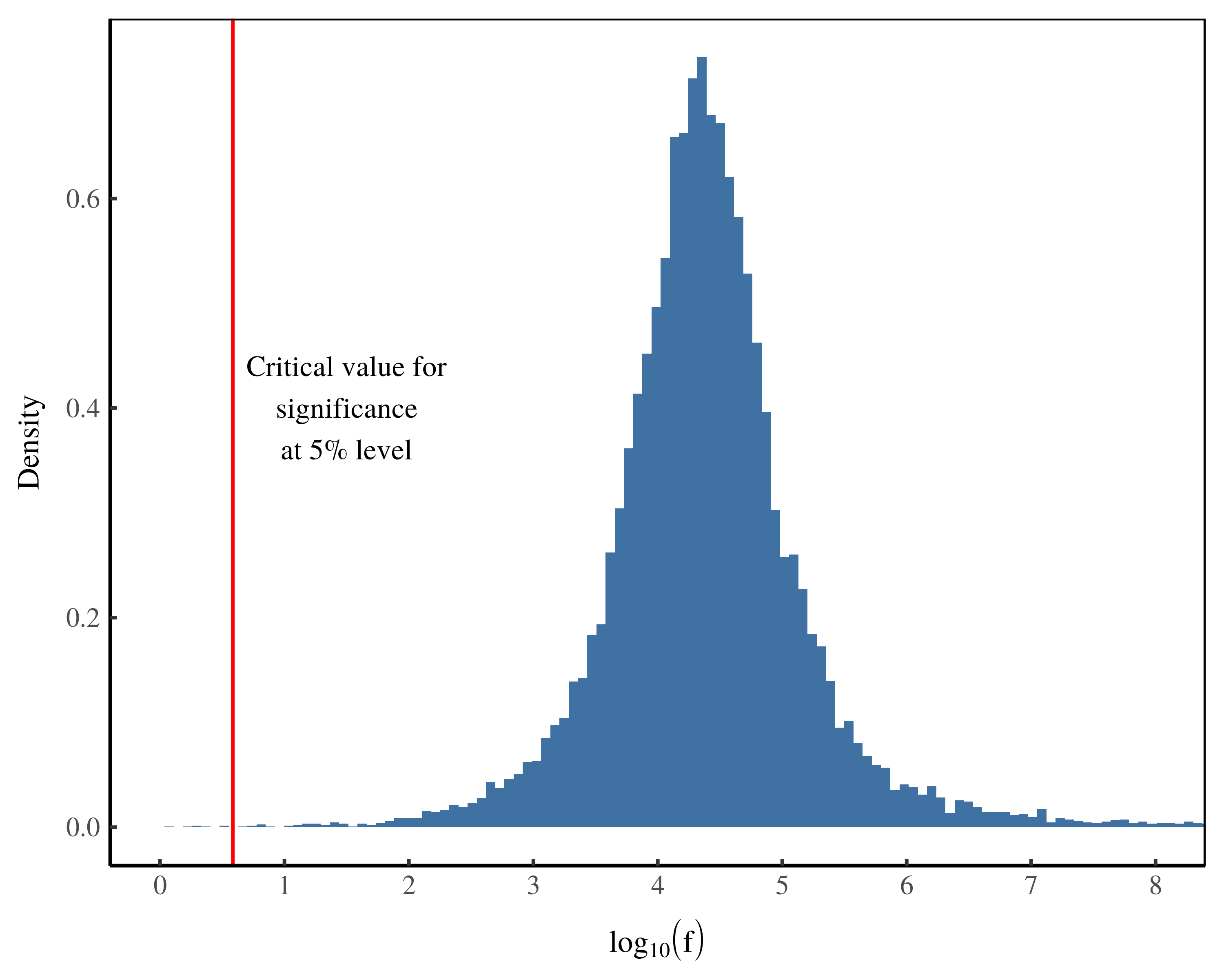
Figure 2 shows yet another way of looking at the simulation results. Instead of plotting p-values, here I look at the distribution of the f-statistic. The f-statistic is another way of measuring ‘statistical significance’ (p-values are actually derived from the f-statistic). But whereas a lower p-value is ‘more significant’, a higher f-statistic is ‘more significant’.

As with p-values, the f-statistics are so extreme that I need to plot their logarithm. The vertical red line in Figure 2 shows the threshold for statistical significance at the 5% level. Results with an f-statistics above this value are deemed ‘statistically significant’. Again, we see that the vast majority of results are ‘statistically significant’.

It seems that by throwing random numbers into our accounting definition, we can’t help but find a correlation between wages and value added per worker.

Manufacturing correlation

The charge that I’ve laid against neoclassical economists is that when they test their theory of income, they’re fooling themselves. Their method (virtually) guarantees a positive result. They regress two types of income — wages and value added per labor hour — that are related by an accounting definition. The problem is that this accounting definition (virtually) guarantees a statistically significant correlation.

Now the degree to which this correlation is guaranteed depends on the specifics of how the wage bill, profit and labor hours are distributed. But what I’ve shown here is that across a huge class of numbers, a ‘statistically significant’ correlation is almost unavoidable. It’s manufactured by our accounting definition.

This result highlights a problem with how economists use p-values. The use of p-values has turned into a production function: run a regression → get a low p-value → get published. Rarely do economists question whether the assumptions behind p-values are actually met in the real-world data.

In my simulation, the assumptions behind p-values are systematically violated. To use them, we must assume that our data is ‘statistically independent’. Here, this means that wages and value added per labor hour can be treated as independent, random variables. The problem is that they’re not independent. Wages and value add per labor hour are related by an accounting definition. This renders them highly dependent. So the use of p-values is moot.

Still, p-values are the standard by which economists judge correlation. By this standard, our accounting definition virtually guarantees a ‘statistically significant’ correlation between wages and value added per labor hour.

The larger problem

The larger problem here is that the marginal productivity theory of income is untestable. Its core components — productivity and the ‘quantity’ of capital — cannot be measured objectively. If you want to know more about these problems, I recommend John Pullen’s book The Marginal Productivity Theory of Distribution: A Critical History.

The reality is that when it comes to explaining income, there is a long and sordid history of political economists fooling themselves. Neoclassical economists may be the most visible fools, but they’re by no means the only ones. Marxists too test their theory of income in circular terms. If you’re interested in Marxist theory, check out the debate between Jonathan Nitzan, Shimshon Bichler and the Marxist Paul Cockshott. What appears to be evidence for the labor theory of value, Nitzan and Bichler show, is actually mathematical foolery.

This issue of circular testing cuts to a core problem in both neoclassical and Marxist theories of income. Both explain income in terms of quantities that are unobservable. Unsurprisingly, tests of these theories resort to circular logic. Such tests invariably show that two forms of income are correlated. Then they claim that one form of income is something other than what it seems.

Sadly, this foolery has been standard practice for a century. And that’s not really surprising. There is perhaps no topic in which objectivity is more difficult than the distribution of income. Still, if we want a scientific theory of income, we need to do better. We need to stop fooling ourselves.

Notes

Here’s my model. I assume that profit (P), the wage bill (W) and the number of labor hours (L) in firms are random variables that are lognormally distributed. If you’re not familiar, the lognormal distribution looks like a bell curve when you take the logarithm of its values. If the variable x is lognormally distributed, log(x) is normally distributed. Many quantities in economics are lognormally distributed, which is why I use this function here.

The lognormal distribution has two parameters, the ‘location’ parameter mu and the ‘scale’ parameter sigma. I’ll denote the lognormal distribution with the notation used in R. If x is lognormally distributed with parameters mu and sigma, I denote it as:

x = lnorm(mu, sigma)

To assume almost nothing about the distribution of P, W and L, I let the parameters of the lognormal distribution vary randomly over a uniform distribution. I’ll denote the uniform distribution using the notation used in R. If x is a uniformly distributed over the range 0 to 1, we write:

x = runif(0, 1)

I let the parameters of the lognormal distribution vary between 0 and 10. If you’re familiar with the lognormal distribution, you’ll know that this is a huge parameter space. So the values of P, W and L are:

P = lnorm( mu = runif(0, 10), sigma = runif(0, 10))

W = lnorm( mu = runif(0, 10), sigma = runif(0, 10))

L = lnorm( mu = runif(0, 10), sigma = runif(0, 10))

I take these values and throw them into the accounting definition. Average wages are then W / L. Value added per worker is (W + P) / L. To see how the correlation between wages and value added per worker varies, I run the algorithm several thousand times.

Code

Here’s the R code for the model. Run it for yourself and see what you find.

library(doSNOW)

n_test = 20000
n_firms = 10^4

# cluster
cl = makeCluster(4, type="SOCK")
registerDoSNOW(cl)
clusterSetupRNG (cl, type = "RNGstream")

# progress Bar
pb = txtProgressBar(max = n_test, style = 3)
progress = function(n) setTxtProgressBar(pb, n)
opts = list(progress = progress)

test = foreach(i = 1:n_test, .options.snow=opts, .combine=rbind)  %dopar%  {
    
    # wagebill
    mu = runif(1, 0, 10)
    sigma = runif(1, 0, 10)
    wagebill = rlnorm(n_firms, mu, sigma)
    
    # profit 
    mu = runif(1, 0, 10)
    sigma = runif(1, 0, 10)
    profit = rlnorm(n_firms, mu, sigma)
    
    # value added (sum of wagebill and profit)
    value_added = wagebill + profit
    
    # labor hours
    mu = runif(1, 0, 10)
    sigma = runif(1, 0, 10)
    labor_hours = rlnorm(n_firms, mu, sigma)
    
    # hourly wage
    hourly_wage = wagebill / labor_hours
    
    # valued added per labor hour
    va_per_hour = value_added / labor_hours

    # regress value added per hour and hourly wage
    r = lm( log(va_per_hour) ~ log(hourly_wage) )
    
    f = summary(r)$fstatistic
    
    f_stat = f[1]
    p = pf(f[1],f[2],f[3],lower.tail=F)
    r2 = summary(r)$r.squared
  
    output = data.frame(f_stat, p, r2)
    
}
stopCluster(cl)

# portion that are significant
sig_frac =  length(test$p[ test$p < 0.05 ]) / length(test$p)

# f statistic
hist(log10(test$f_stat), breaks = 100, xlim = c(0, 10))
abline(v = log10(3.85), col = "red" )

# export
write.csv(test, "test_data.csv")

Further reading