What Trait Affects Income the Most?

What Trait Affects Income the Most?

January 5, 2021

Originally published on Economics from the Top Down

Blair Fix

If the history of science has taught us anything, it’s that we can’t trust our preconceptions about how the world works. All human societies have developed stories about their place in the cosmos. Almost without exception, these stories were wrong.

True, we’ve killed many of the old myths. But the process was slow and excruciating. Humans have existed for hundreds of thousands of years. Yet it’s only in the last 0.1% of our existence that we’ve discovered the truth (we think) about our place in the cosmos.

This revolution in our knowledge comes down to one thing: evidence. As we looked closely at the cosmos, our origin stories became increasingly tenuous. They simply could not explain the evidence. And so, with great effort, we abandoned these stories (many of us, anyway).

Why is it so difficult to abandon old myths? One reason is that these myths are used to rationalize social order. Take, as an example, the Earth’s orbit. It took the Catholic church nearly 400 years to admit that the Earth revolves around the sun. Why so long? Because the church’s power was at stake. The church tied its dogma — and hence its authority — to a geocentric view of the universe.

Faced with a challenge to its authority, the church acted predictably. After convicting the heliocentric proponent Galileo of heresy in 1633, the church banned heliocentric teachings for another two centuries (until 1822). It took another 170 years for the church to formally admit (in 1992) that Galileo was right. Think about that. Almost four centuries of denial for an idea that had no effect on daily life. All because it threatened the authority of those with power. The lesson here is simple. When ideas challenge authority, evidence will be ignored, denied and suppressed.

That brings me to economics.

The discipline of economics is the modern equivalent of the church. To legitimize authority, neoclassical economists preach dogmas that are manifestly false. But unlike the ethereal debate about the Earth’s place in the cosmos, economic dogmas have a huge impact on day-to-day life. They make the difference between tolerating inequality versus being enraged by it.

Neoclassical economics preaches that all is fair with the distribution of income. Income differences, the theory claims, stem from differences in productivity. As long as markets are competitive, people earn their ‘marginal product’. And so there’s no reason to redistribute income.

The reality is quite different. Income, I believe, is determined not by productivity, but instead largely by rank within a hierarchy. In other words, power begets income. The role of economics is to deny this uncomfortable reality. Economists reinforce hierarchies by denying their existence.

As Galileo showed, the way to combat dogma is to confront it with evidence. With that in mind, I’m going to show you evidence that challenges the neoclassical faith. Looking at the United States, I find that the single most important determinant of income is something that neoclassical economists refuse to study. It’s not education. It’s not occupation. It’s hierarchical rank.

Measuring effect size

Here’s the road ahead. I’m going to make a list of different human traits. Then I’m going to measure how strongly each trait affects income. But before we get to the evidence, we need to talk statistics. What does it mean for a trait to have a ‘large’ effect on income? Conversely, what does it mean for a trait to have a ‘small’ effect on income? How do we measure this effect size?

Here’s what statisticians have proposed. To measure effect (on income, or anything else) we compare variation between groups to variation within groups. If a trait has a large effect on income, the income differences between trait groups should dwarf the differences within groups. Conversely, if a trait has a small effect on income, the income differences within trait groups should dwarf the differences between groups.

To get an intuitive understanding for this measure of effect size, we’ll begin with something more immediate than income. Let’s step on the scale and see what affects human weight. We’ll use Americans as our guinea pigs.

A small effect

Americans tend to grow heavier with age — likely due to the obesity epidemic. But while this epidemic is devastating to human health, weight gain with age is actually quite small. Figure 1 shows the data. Here I plot the mass distribution of two groups of Americans: those ages 18–24, and those ages 65 or older. You can see that seniors are slightly heavier than young adults. But the effect is small. (You may be complaining that I’m not tracking the same cohort over time, so I can’t judge trends. Fair point. But my purpose here isn’t to rigorously study weight gain. It’s to visualize effect size.)

How do we quantify the size of this age-weight effect? To measure effect size, we compare weight differences between groups to weight differences within groups.

Let’s start with differences between groups. In Figure 1, the vertical lines show the average weight of each cohort. American seniors weigh on average 79 kg. Americans age 18–24 are slightly lighter, weighing on average at 76 kg. So seniors are about 3 kg heavier (on average) than their younger counterparts.

Now we ask — is this 3 kg difference large or small? The answer depends on variation within each cohort. Before getting to the math, think about it this way. If I was comparing the mass of two types of ant, a 3 kg difference would be huge. But if I was comparing the mass of two types of elephant, a 3 kg difference would be tiny. The difference between groups gains meaning only when compared to variation within the group.

To measure variation within groups, we’ll use the standard deviation. This measure quantifies the relative spread of the distribution. The larger the standard deviation, the greater is the variation within the group. Looking at our age cohorts, we find that the standard deviation within each group is about 19 kg. Compared to this variation within groups, our 3 kg difference between groups is small. You knew this intuitively when you looked at Figure 1 and saw that the two distributions almost completely overlapped. But now we have a metric to quantify your intuition.

A medium-sized effect

Let’s move on to a medium-sized effect. Men are, on average, heavier than women. This effect turns out to be larger than the age-weight effect. Figure 2 shows the data. American men weigh on average 90 kg. Women weigh on average 75 kg. So men are about 15 kg heavier (on average) than women.

How large is this 15 kg difference between sexes? To judge its size, we compare it to the weight variation within each sex (measured using the standard deviation). This within-group variation is about 19 kg. So our 15 kg difference between sexes amounts to almost one standard deviation. In other words, sex has a medium-sized effect on weight.

A large effect

Now let’s move on to a large effect. We’ll compare the weight of adults to the weight of newborns. Figure 3 shows the data. The average American adult weighs 82 kg. The average newborn weighs 3 kg — a difference of 79 kg.

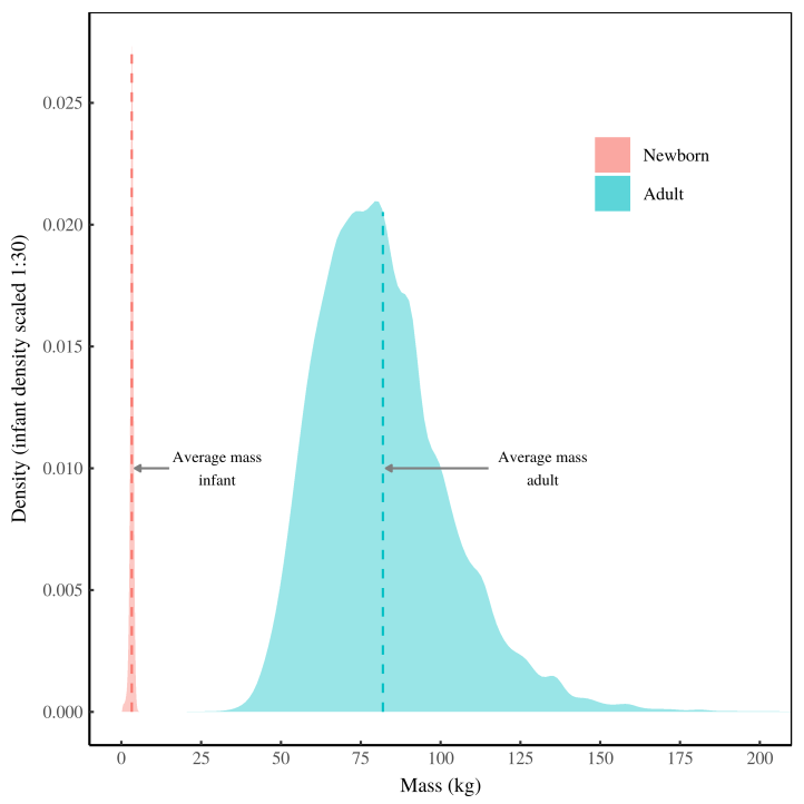
It’s obvious, from Figure 3, that we’re dealing here with a large effect. But let’s quantify it. To do so, we compare the 79 kg difference between newborns and adults to the variation within each group. This variation, measured by the standard deviation, is about 11 kg. So the variation between groups is about 7 times greater than the variation within groups. That’s a large effect.

Comparing the signal to the noise

When we compare variation between groups to the variation within groups, we’re comparing a signal (the effect) to the noise (the non-effect). The ratio of the two is called the signal-to-noise ratio. It’s how we’ll measure effect size.

Table 1 shows the signal-to-noise ratio for how our three traits affect weight. Adult age has a weak effect on weight. Sex has a medium-sized effect. And growing from newborn to adulthood has a large effect. [1]

Table 1: Measuring how traits affect weight

Trait	Difference in average mass (kg)	Average mass variation within groups (kg)	Signal-to-noise ratio
senior vs. young adult	2.7	19.3	0.14
male vs. female	15.5	19.4	0.80
adult vs. newborn	78.7	10.7	7.33

The signal-to-noise ratio in Table 1 is called Cohen’s d. It’s useful when we want to measure an effect between 2 groups. But what if we have many groups? Then we can’t take as the signal the difference between groups (it’s ill-defined for three or more groups). We need another approach.

The solution is to switch from measuring the difference between groups to measuring the variation between groups. If we use the standard deviation to measure this variation, the resulting signal-to-noise ratio is called Cohen’s f. The numerator changes (from Cohen’s d), but the interpretation remains the same. A larger signal-to-noise ratio indicates a larger effect.

When studying effect on income, however, it’s more convenient to use a slightly different signal-to-noise ratio. Income variation is usually reported using the Gini index (not the standard deviation). So it’s more convenient to construct our signal-to-noise ratio using the Gini index.

Here’s how I’ll measure effect on income. I’ll compare the Gini index between groups to the Gini index within groups:

As before, a larger signal-to-noise ratio indicates a greater effect on income. (For more details about the metric, see this paper.)

How traits affect US income

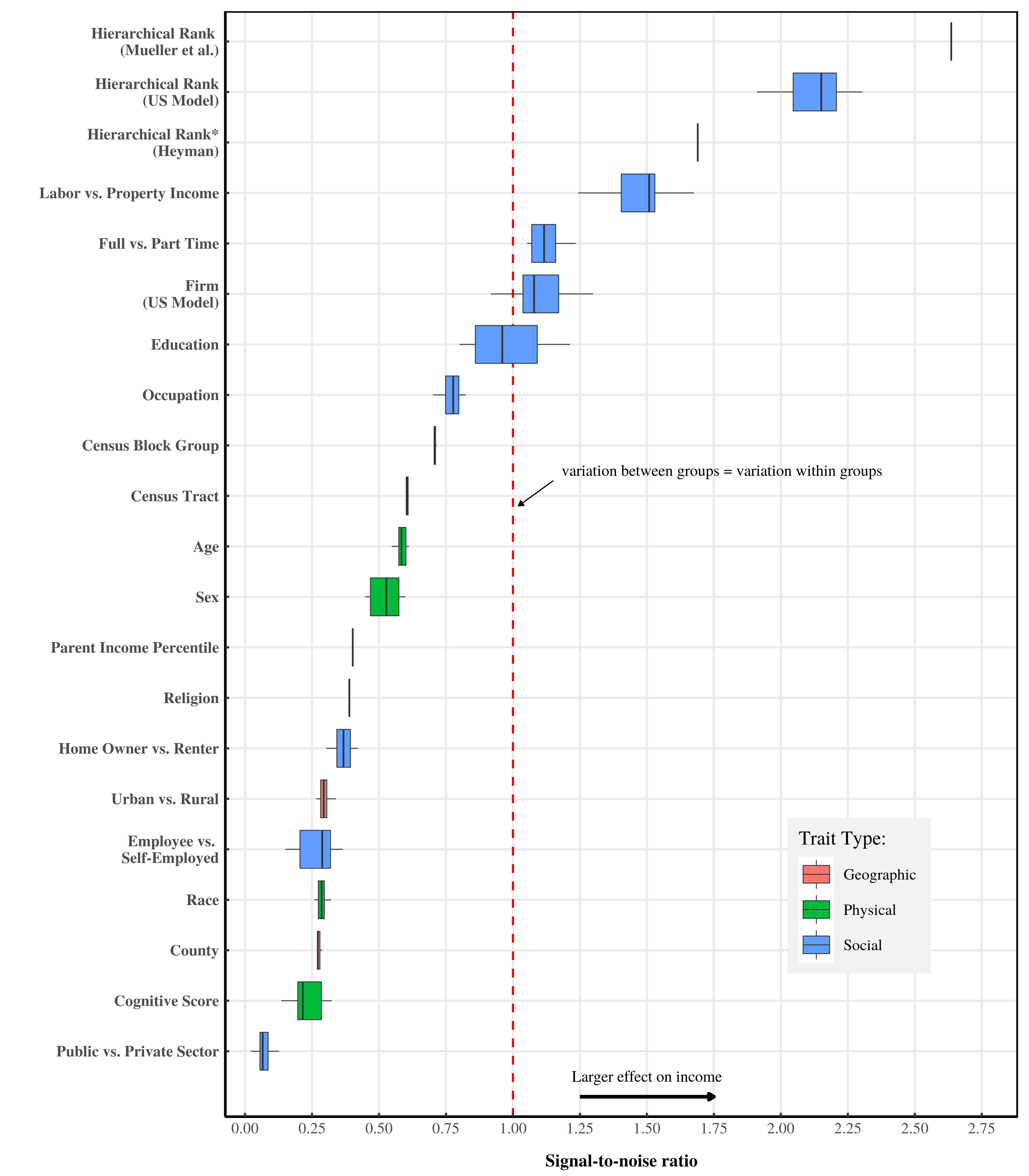
Now that you’ve had a crash course in the statistics of effect size, let’s get to the data. Figure 4 shows how various traits affect the income of Americans. The list of traits isn’t exhaustive. It’s merely the traits for which I could find data. (If you think of a trait that I missed, leave a comment.)

Let’s walk through how to interpret Figure 4. The y-axis shows the various traits. I’ve used color to classify these traits into three types: geographic, physical, and social. The x-axis shows each trait’s effect on income, measured with the signal-to-noise ratio. The boxplots indicate the variation (mostly over the last two decades) in the signal-to-noise ratio. (Here’s how to interpret a boxplot. The vertical line indicates the median of the signal-to-noise ratio. The ‘box’ shows the middle 50% of the data. And the horizontal line shows the data range. A single vertical line indicates that there’s only one data point.)

Physical traits

Now that you understand the chart, let’s walk through the results. We’ll start with physical traits — properties of the individual’s body and brain. These traits have a surprisingly weak effect on income. Take cognitive score (i.e. measured IQ). Americans love to believe that intelligence is rewarded, meaning they live in a meritocracy. Unfortunately, the evidence squashes this myth. Cognitive score, it seems, has a trivial effect on income. [2]

Interestingly, race (as categorized by the US government) also has a weak effect on income. This doesn’t mean that racism isn’t a problem. It’s just that the income difference between races is relatively small compared to the income variation within each race. (Side note: the categorization of race is obviously subjective. The way the US census has classified race has changed over time, reflecting changing politics.)

Moving up the ladder, sex has a stronger effect on income. Women tend to earn less than men. Why? There are probably three reasons. First, women are more likely to work part time. Second, women tend to work at lower-paying jobs. Third, women are generally paid less than men even when they do the same job.

Moving to the top of the ladder, the physical trait with the strongest effect on income is age. That’s easy to understand. Baby boomers, you’ve probably noticed, tend to out-earn millennials. If you believe human capital theory, this happens because people become more skilled (and hence, more productive) with age. But I’m skeptical of this idea. I think that people earn more with age largely because they get promoted in the corporate hierarchy. (We’ll come back to hierarchy in a moment.)

Geographic traits

Let’s move on to geographic traits (i.e. the place where you live). It turns out that geography affects income quite weakly. This finding is somewhat surprising, given the segregated nature of US society. There’s no doubt that the US has rich areas and poor areas. But no matter how you slice up space, the income effect of geography is comparatively small. (Sidenote: it would be interesting to see if this geographic effect was greater when segregation was an official policy, rather than an unspoken norm.)

Looking at the data, it seems that dividing the US into counties has the weakest effect on income. The divide between urban dwellers and rural dwellers is slightly larger. (People in cities tend to outearn their rural counterparts.) As we shrink the geographic area, the effect on income grows. The effect of grouping people by census tract slightly trumps the income effect of age. Shrinking the geographic area to census block groups (the size of a few city blocks) increases the income effect a bit more.

What this result tells us is that US spacial inequality is fine grain. Over large spaces (like counties), income differences are small. But as we shrink down to the city block, income differences grow. If you’ve ever walked through a city like New York, this result makes sense. The transition between a wealthy neighborhood and poor neighborhood can happen in a few hundred feet. While highly visible, this geographic effect on income is dwarfed by the effect of many social traits. So despite the segregation of US society, geography has a fairly weak effect on income.

Social traits

If humans were solitary animals, we’d expect that physical and/or geographic traits would affect income the most. (The lone wolf that’s bigger or has better territory gets more resources.) But humans are not solitary animals. We’re a social species. As such, we expect that social traits should most strongly affect income.

The US evidence confirms this expectation. The 6 traits with the largest effect on income are all social. And social traits are the only ones to cross the one-to-one threshold in our signal-to-noise indicator. In other words, they’re the only traits that have a ‘large’ effect on income.

Let’s discuss these 6 traits with the largest effect on income. We’ll start with occupation. It’s a fact of life that some jobs pay more than others. Doctors earn more than janitors. Lawyers earn more than nurses. Why this happens is matter of debate. If you’re a neoclassical economist, you’d say that lawyers have more human capital than nurses. (Interestingly, few economists have the guts to state this bluntly in the current pandemic.)

If you don’t believe the neoclassical fantasy, you’d probably say that there’s many factors at work. Better-paying jobs are often protected by guilds that maintain a barrier to entry. Poor-paying jobs are open access. Good-paying jobs are often unionized. Minimum-wage jobs are not. Some jobs are prestigious, others are not. And perhaps most importantly, some jobs (like CEO) are at the top of the corporate hierarchy. Others are at the bottom. I could go on, but you get the point. There’s probably many reasons that income varies by occupation.

Let’s move up the effect-size ladder to education. It’s worth pausing here to discuss the role of education in the neoclassical theory of income. According to human capital theory, training (of any kind) makes you more productive, and hence earn more income. The most obvious type of training is formal education. In 1958, neoclassical economist Jacob Mincer proposed that years of formal education could explain individual income. Since then, Mincer’s approach has become neoclassical gospel.

The problem (which Mincer himself discovered) is that education can’t explain income. The correlation between income and education is actually quite small. Here’s Mincer writing in 1974:

Simple correlations between earnings and years of schooling are quite weak. Moreover, in multiple regressions when variables correlated with schooling are added, the regression coefficient of schooling is very small.

Now, on its own, this low correlation between income and education isn’t fatal to human capital theory [3]. The fact is that most traits weakly affect income. This is evident in Figure 4. The income effect of most traits is well below the one-to-one level (meaning within-group variation trumps between-group variation). So yes, income is weakly correlated with education. But as long as education has the strongest effect on income, there’s no fatal blow to human capital theory.

The problem is that education doesn’t have the strongest effect on income — not even close. The income effect of education is dwarfed by the effect of hierarchical rank (discussed in detail below). So it seems that human capital theorists have hitched their train to the wrong trait.

Let’s move further up the effect-size ladder. Firm membership, I find, is the first trait to pass the one-to-one threshold in our signal-to-noise indicator. This means that income variation between firms is greater than income variation within firms. What this means is that, regardless of your position, you’ll tend to earn more at Goldman Sachs than at McDonald’s. The caveat here is that this estimate is based on a model. So treat it with appropriate uncertainty. (For details about the model, see this paper.)

Let’s move up the effect-size ladder again. Working full time versus working part time strongly affects income. This finding is easy to understand. Part-time employees work fewer hours than their full-time counterparts. And part-time wages also tend to be worse.

Moving up one more effect-size rung and we get to labor versus property income, which very strongly affects income size. You may think that this large effect happens because property owners (i.e. capitalists) tend to outearn workers. But it’s actually the reverse. The average property owner earns far less than the average worker.

What’s going on here? This result has to do with how property income is distributed. The vast majority of property owners earn almost nothing — a few dollars in interest from their savings account, and some meager dividends on their investments. For most people, this is hardly enough to survive on. That’s why they work. Sure, there are people like Bill Gates who earn all their income from property. But these people are exceedingly rare. Because most property owners earn almost nothing, labor income tends to dwarf property income.

If you’re a Marxist, this result should give you pause. Formulated in the 19th century, Marxist theory envisions a clean division between capitalists and workers. In reality, no such division exists. Most people earn a tiny bit of capitalist income. A few people earn a lot. So being a capitalist (or not) is a matter of degree. (As an aside, it turns out that this degree of being a capitalist is closely related to hierarchy. I discuss how here.)

The effect of hierarchy

We’ve finally arrived at the raison d’être of this post — the income effect of hierarchy. My hypothesis is that hierarchy is central to how humans distribute resources. The reasoning is simple. Our social relations govern how we divide the pie. And hierarchical relations are by far the most potent. The testable consequence of this hypothesis is that hierarchical rank should effect income more strongly than any other trait.

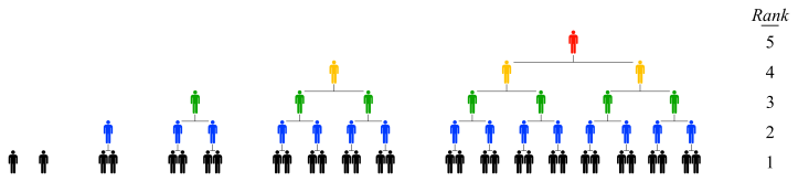
Before getting to the results, I’ll clarify what it means to group individuals by hierarchical rank. Figure 5 shows a conceptual example. Here we have different hierarchies, with distinct hierarchical ranks. To measure the income effect of hierarchical rank, we group people by rank across all hierarchies.

In conceptual terms, it’s easy to measure how hierarchical rank affects income. But in practical terms, it’s quite difficult. The problem is that few people have gathered the relevant data. Although ubiquitous in human societies, hierarchy has not been well studied.

To estimate how hierarchical rank affects income, I cobble together three different sources. Each source comes with caveats, and none are ideal. The data labeled ‘Mueller et al.’ (in Figure 4) comes from a study of UK firms. The data labeled ‘Heyman’ comes from a study of Swedish firms, and carries the ‘*’ because it doesn’t include all hierarchical ranks within firms. The data labeled ‘US model’ is a model-based inference, based jointly on data from firm case studies and the pay of US CEOs. (For details about the model, see this paper.)

This data on hierarchy is admittedly ragtag. But that’s part of wading into uncharted empirical territory. What’s important here are two things. First, despite their ragtag nature, the three estimates for the income effect of hierarchy are consistent with one another. Second, these estimates dwarf the effects of all other traits.

So the evidence, which is admittedly uncertain, suggests that hierarchical rank has the strongest effect on income.

And yet it moves

Upon being convicted of spreading heresy, Galileo is said to have remarked: “And yet it moves.” He was referring of course, to the Earth. Galileo had mustered the first evidence that the Earth revolves around the sun. The evidence, though, was indirect. Galileo had closely watched the motion of Venus, and found that it had phases — just like the moon. He concluded that this could happen only if Venus orbited the Sun. By extension, he inferred that the Earth also moved around the Sun.

The Church thought differently. Of the heliocentric model, the church inquisitors concluded:

… this proposition is foolish and absurd in philosophy, and formally heretical since it explicitly contradicts in many places the sense of Holy Scripture …

New evidence, unfortunately, is often greeted with this reaction — especially by people with a lot (of power) to lose. While my research pales in comparison to Galileo’s, it’s been greeted with similar resistance. ‘Formally heretical’ … ‘contradicts scripture’. This is essentially the reaction to Figure 4 that I’ve received from neoclassical economists.

Now, I’m the first to admit that the evidence is uncertain. Moreover, this evidence doesn’t establish causation. It doesn’t tell us that hierarchical rank causes income. Still, the evidence suggests that something is deeply wrong with the neoclassical understanding of income. It suggests that treating hierarchical rank as the strongest determinant of income is a hypothesis worth exploring.

Neoclassical economists will have none of this. The idea that hierarchical rank most strongly affects income, I’ve been told, is ‘foolish and absurd’. Why? Because it explicitly contradicts neoclassical scripture. Income, scripture says, must stem from productivity. So behind hierarchical rank, there must lurk some unmeasured skill. Silly me — I’m naive enough to take my results at face value, just as Galileo did when interpreting the phases of Venus.

The case for hierarchy’s effect on income is tentative, yes. But if we accept dogma, we’ll never know the truth. The task for hard-nosed scientists is to gather more evidence and see what happens. Either the case will grow stronger with more evidence, or it will disappear. Join me in this search.

Notes

[1] Whether we call an effect ‘large’ or ‘small’ is arbitrary. It depends on the type of phenomena we’re studying. In psychology (where effect sizes are generally small), the common thresholds for Cohen’s d are: small effect = under 0.2, medium effect = between 0.2 and 0.8, large effect = over 0.8. When it comes to income, my preference is that we shouldn’t call an effect ‘large’ unless the variation between groups is larger than the variation within groups. This threshold corresponds to a signal-to-noise ratio larger than 1.

[2] Is cognitive score a ‘physical’ trait? I use the term ‘physical’ here not in a genetic determinist sense, but in the sense of ‘residing in the person’s body’. Every property of the brain, whether inborn or learned, is a ‘physical’ trait because it’s a property of the matter inside the person. (OK, this isn’t true if you believe in mind-body dualism.) There’s no doubt that practice can improve your performance on IQ tests, in the same way that exercise can improve your athletic performance. But both types of performance still reside in the body.

[3] There are many other blows to human capital theory that are fatal. Most importantly, the theory posits that productivity explains income. But economists never measure productivity independently of income. Instead, all of their evidence for productivity is, in fact, circularly tied to income. For details, see these posts: No, Productivity Does Not Explain Income, Productivity Does Not Explain Wages, Debunking the ‘Productivity-Pay Gap’, and Productivity and Income … Again.

Further reading