The Buy-to-Build Indicator: New Estimates for Britain and the United States

The Buy-to-Build Indicator

New Estimates for Britain and the United States

JOSEPH A. FRANCIS

October 2013

Abstract

This note presents new long-term estimates of what Jonathan Nitzan and Shimshon Bichler have named the ‘buy-to-build indicator’, which is calculated as the value of mergers and acquisitions as a percentage of gross capital formation.

Keywords

Britain, buy-to-build indicator, mergers and acquisitions, United States

Citation

Joseph A. Francis (2013), ‘The Buy-to-Built Indicator: New Estimates for Britain and the United States’, Review of Capital as Power, Vol. 1, No. 1, pp. 63-72.

Download PDF

This note presents new long-term estimates of what Jonathan Nitzan and Shimshon Bichler (2009: Ch. 15) have named the ‘buy-to-build indicator’, which is calculated as the value of mergers and acquisitions as a percentage of gross capital formation. According to Nitzan and Bichler (2009: 338), ‘this index corresponds roughly to the ratio between internal and external breadth’, which are two of the four ‘sub-routes’ that dominant capital takes to ‘accumulate differentially’ (2009: 329). Expenditure on mergers and acquisitions indicates how much is being invested in already-existing assets, while gross capital formation is roughly equivalent to green-field investment (that is, investment in new productive capacity). The ratio between the two — the buy-to-build indicator — thus shows which of these two ways of expanding is most prominent at a particular moment in time.

It is Nitzan and Bichler’s (2009: 331, 338-39, 359) contention that buying has increasingly come to predominate over building since the late nineteenth century because buying already existing capacity reduces the risk of glut, whereas building new capacity increases it. Consequently, they argue, capitalism has seen a tendency ‘for chronic stagnation to gradually substitute for cyclical instability’ (2009: 331), as corporate amalgamation has become the ‘main engine of differential accumulation’ (2009: 332). Only when some temporary barrier to further amalgamation is met does the wave of amalgamation subside, typically leading to a period of stagflation, as dominant capital instead accumulates differentially through ‘external depth’, which occurs through stagflation, as dominant capital limits production, in order to redistribute income in their favor through inflation. These pendular swings from external depth to external breadth and back again provide the basic rhythm of the capitalist mode of power. It is important, therefore, that they are correctly measured.

This note provides two new series of buy-to-build indicators. Estimating them, it should be stressed, is not simple, principally due to the absence of consistent series for expenditure on mergers and acquisitions. Nevertheless, as this note describes, it has proven possible to calculate them for both Britain and the United States. For Britain, the new estimates build principally on the research of Leslie Hannah (1983), as well as official government statistics, while for the United States, they represent significant revisions of Nitzan and Bichler’s own original estimates. The note concludes with some observations on the new series, including on how they affect (or not) Nitzan and Bichler’s narrative.

New Estimates

Britain

Estimating a buy-to-build indicator for Britain is relatively straightforward. Hannah’s (1983: 167-78) series of the value of firm disappearances due to mergers and acquisitions in manufacturing industry during 1880-1939 and 1949-1981 can be easily spliced with the official Office for National Statistics (ONS n.d.: Series DUCM and CBCQ) series of expenditure on mergers and acquisitions, which covers expenditure on mergers and acquisitions in Britain by British companies during 1965-85 and by British and foreign companies in Britain during 1986-2012. The raw data can be seen in part (a) of Figure 1, in which the series for the value of mergers and acquisitions are shown as percentages of gross fixed capital formation,¹ in order to arrive at buy-to-build indicators.

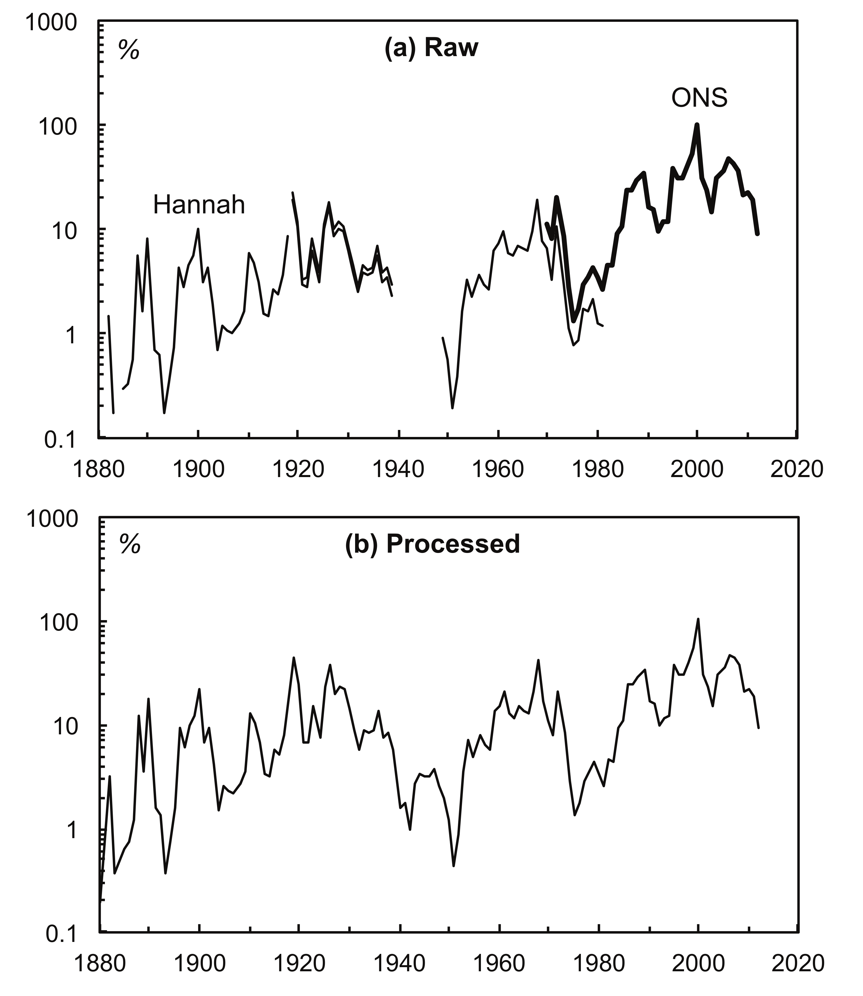Figure 1: Raw and Processed Buy-to-Build Indicators for Britain.
Note: Logarithmic scale. Sources: See text.

Simple ratio splicing was used to join the Hannah and ONS series. Hannah’s series was adjusted upwards according to the average ratio between the two during 1965-81, in order to roughly compensate for the absence of non-manufacturing mergers and acquisitions in Hannah’s series. During 1919-39, Hannah gives low and high estimates of the value of mergers and acquisitions in manufacturing, so the average of the two was used. The gap in Hannah’s series between 1939 and 1949 was filled through exponential interpolation, adjusted following the variations in a proxy that was construct by multiplying the number of mergers and acquisitions by the Actuaries General Share Price Index, then dividing it by gross fixed capital formation.² The continuous buy-to-build indicator that resulted from this processing can be seen in part (b) of Figure 1.

The United States

Constructing a series for the United States is more difficult because the data on mergers and acquisitions are less consistent and somewhat scarcer.³ Seven sources can be identified:

Luther Conant’s (1901: 12) series for industrial companies during 1887-1900, covering those acquired worth over US$1 million, according to the total value of all their stock and bonds. Conant’s sources are unclear.
Ralph Nelson’s (1959: 145, 154, Tables B-3 & B-7) series for the manufacturing and mining sector during 1895-1920, based on reporting in the financial press, which tended to underreport smaller mergers and acquisitions.
Carl Eis’s (1969: 271, Table 1) series for industrial companies during 1919-30, covering consolidations worth at least US$1 million and acquisitions of US$100,000 or more, produced under the supervision of Nelson and using a similar methodology.
The Federal Trade Commission (FTC 1981: 104, Table 15) series for the manufacturing and mining sectors during 1948-79, in which the book value of the acquired firm’s assets were US$10 million or more. The US$10 million cut-off creates a major problem for the consistency of this series.
A series for 1968-2007 begun by W.T. Grimm & Co and subsequently published in Mergerstat Review (1991; 2008). The series covers all merger and acquisition announcements in the United States and by US companies abroad, including divestitures, and leveraged buy-outs. The series covers deals worth at least US$500,000 and is limited to only those mergers and acquisitions in which the value was made publicly available.⁴
A series published in the Statistical Abstract of the United States, covering the period 1984-2003 and including ‘mergers, acquisitions, acquisitions of partial interest that involve a 40% stake in the target or an investment of at least [US]$100 million, divestitures, and leveraged transactions that result in a change in ownership’ (US Bureau of the Census 1994: 551; also 2002: 493; 2004-05: 741). The source of these data was the Securities Data Company, which would later become Thomson Financial, and, as in the Mergerstat series, is limited to mergers and acquisitions in which the value was publicly announced.
Thomson Financial’s raw data on mergers and acquisitions, accessed through Thomson ONE Banker. All mergers and acquisitions in which the purchased company was located in the United States were included, while the total value of mergers was treated as the sum of all the announced values of each deal completed in each year.⁵ Again, the major limitation is that it only includes deals in which the value was announced.

Once these series were compiled, each was divided by a series for gross fixed capital formation,⁶ leading to six separate buy-to-build indicators. The results can be seen in part (a) of Figure 2.

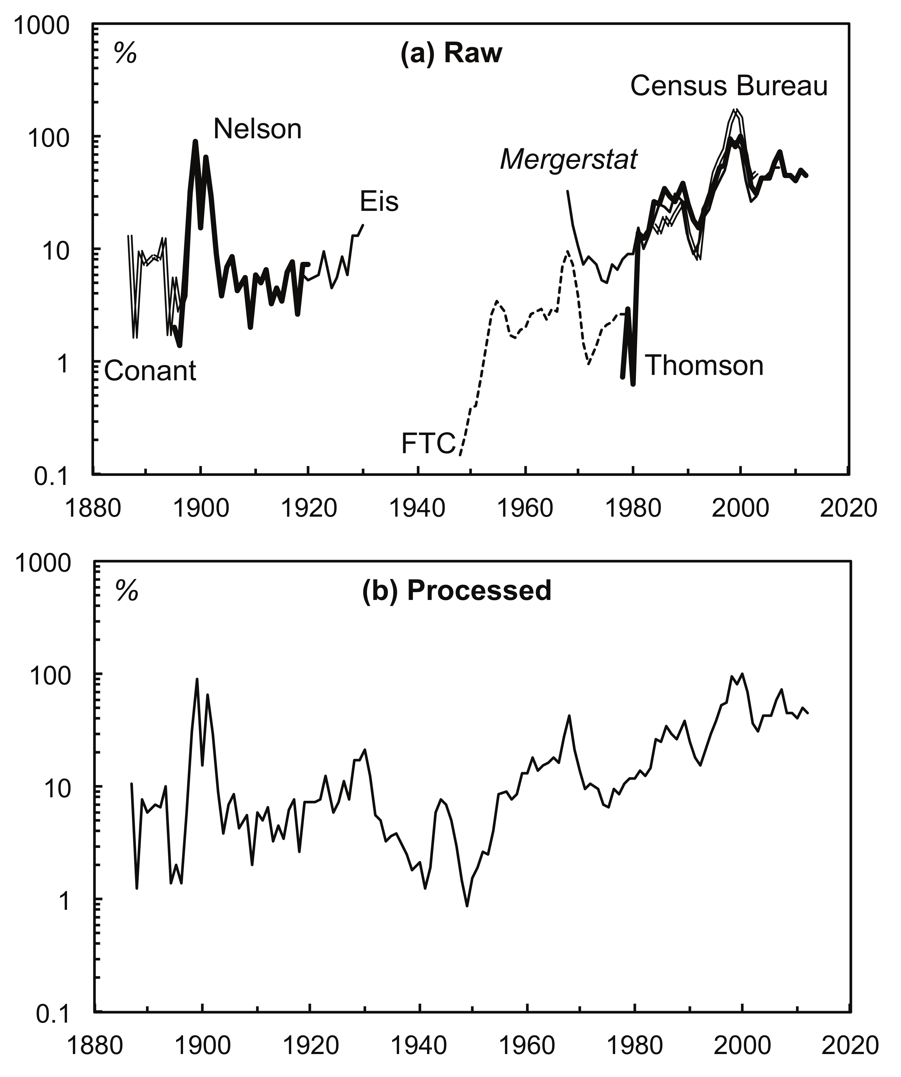Figure 2: Raw and Processed Buy-to-Build Indicators for the United States.
Note: Logarithmic scale. Sources: See text.

Processing the various separate buy-to-build indicators was more complicated than in the case of Britain. Two series were used as bases. First, the indicator calculated from Nelson’s estimates for 1895-1920 was taken as a base, then extended to cover 1887-1930 using the Conant and Eis indicators, adjusted according to their average ratios with Nelson’s series during their overlapping periods. Second, the Thomson indicator was used for 1981-2012,⁷ then extended back to 1968 using the Mergerstat Review series, again adjusted according to their average ratios with the Thomson indicator. The result was two series, covering 1887-1930 and 1968-2012 respectively. Interpolation to cover the gap between the two series was carried out in the same way as for Britain: exponential interpolation adjusted according to variations in a series of the number of mergers and acquisitions multiplied by a share price index,⁸ divided by the series for gross fixed capital formation. The result was the processed series shown in part (b) of Figure 1.

Observations

Three main observations on the new series can be made:

The series for the United States differs considerably from that of Nitzan and Bichler (2009: 338, Figure 15.2), which appear to show a fairly continuous exponential trend from the late nineteenth century to the 2000s. By contrast, the new series is effectively trendless until after the Second World War, when a strong upward trend begins. This difference is principally because of an error in Nitzan and Bichler’s calculations, as they appear to have accidentally used figures for gross fixed capital formation in ‘constant’ 1929 prices up to 1928.⁹ Prices in 1929 were notably inflated compared to the current prices of previous years, resulting in an artificially low buy-to-build indicator. Once the correct current prices are used, as in the new series, the buy-to-build indicator appears higher prior to 1929, doing away with the long-term upward trend. From this perspective, the Great Merger Wave of the 1890s appears truly great, as the buy-to-build indicator would not return to such levels until around the year 2000. Nitzan and Bichler’s (2009: 331) proposition that ‘[o]ver the longer haul, mergers and acquisitions tend to rise relative to green-field investment’ therefore becomes more problematic, with much depending on what qualifies as the ‘longer haul’. It suggests that a more nuanced historical narrative is required.
There is a notable similarity between the British and US buy-to-build indicators, with both following similar patterns: essentially trendless up to the Second World War, with a strong upward trend thereafter. During 1887-2012 the Pearson correlation coefficient between the two series is 0.75, indicating a fairly close correlation. Capitalism, at least in the Anglo-Saxon countries, thus appears to have moved to similar rhythms on both sides of the Atlantic.
For both countries, the buy-to-build indicator has some correlation with Nitzan and Bichler’s (2009: 384, Figure 17.1) ‘Stagflation Index’, which they calculate as ‘the average of: (1) the standardized deviations from the average of the rate of unemployment; and (2) the standardized deviation from the average rate of inflation of the GDP implicit price deflator’. In Figure 3 the correlation can be seen in simple visual terms, as the Stagflation Index and the buy-to-build indicators tend to fluctuate in opposite directions.¹⁰ This could be taken as confirmation of their claim ‘that, following the initial emergence of big business at the turn of the twentieth century, internal breadth and external depth tended to move counter-cyclically’ (2009: 385). Figure 3 suggests that this has been the case not only in the United States, but also in Britain.

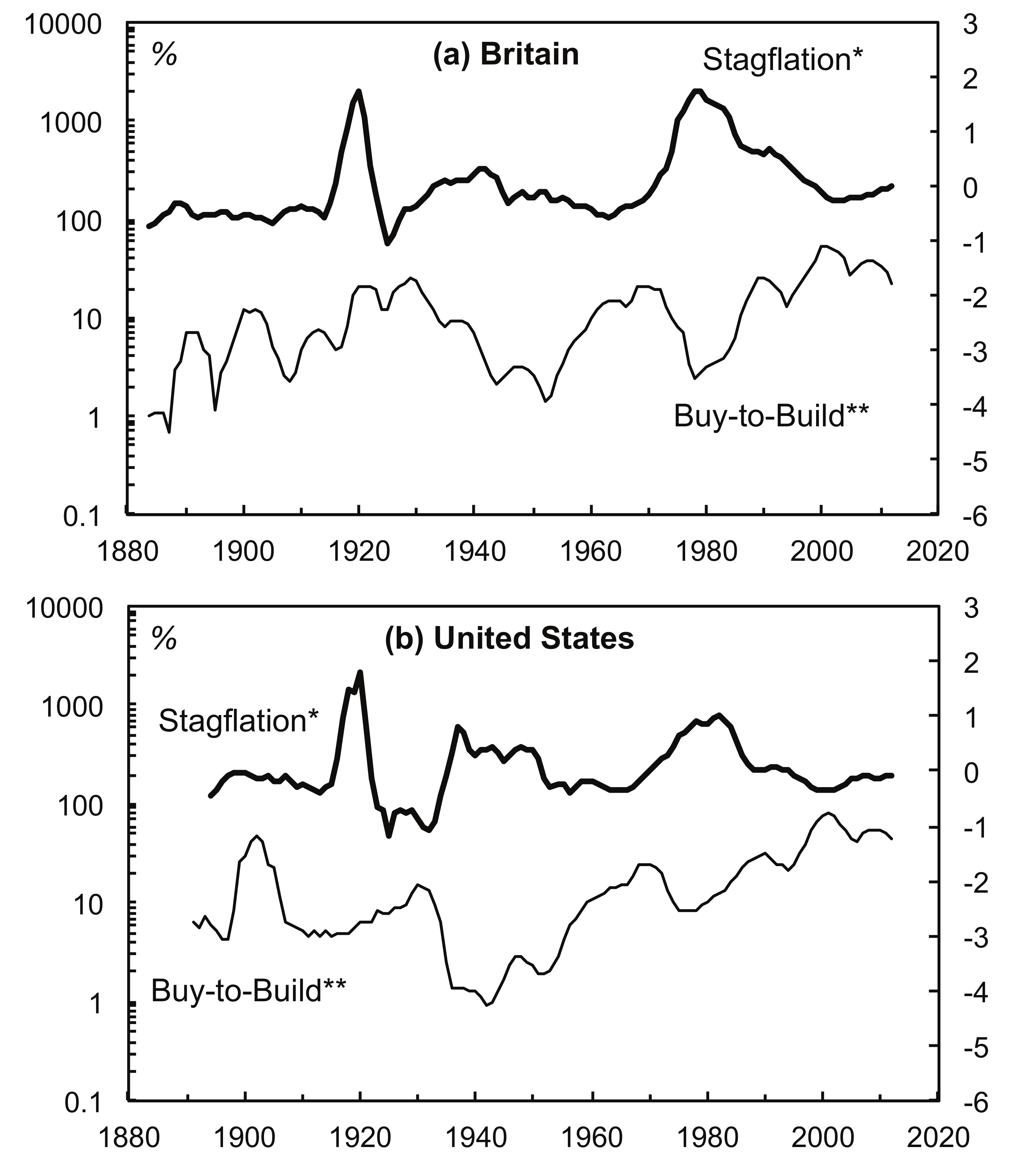
Figure 3: Amalgamation versus Stagflation in Britain and the United States.
* The average of: (1) the standardized deviations from the average of the rate of unemployment; and (2) the standardized deviation from the average rate of inflation of the GDP implicit price deflator. The deviations were standardized by deducting from each year the arithmetic mean of the series over the whole period, then dividing them by the same arithmetic mean.

** Expenditure on mergers and acquisitions as a percentage of gross fixed capital formation.

Note: Both series are smoothed as backward-looking 5-year moving averages. The lefthand axes are shown on a Logarithmic scale. Sources: See text.

Notes

Joseph Francis is a Ph.D. candidate in Economic History at the London School of Economics. This note draws on research that has been supported financially by the Economic and Social Research Council and the London School of Economics. Jonathan Nitzan and Roman Studer commented on an earlier version, although neither is responsible for any errors that remain. The workbook with the raw data and processing described is available at http://joefrancis.info/databases/Francis_buy_to_build.xlsx.

References

BEA (Bureau of Economic Analysis) (n.d.) ‘National Income and Product Accounts’ (http://www.bea.gov/national/nipaweb/index.asp, accessed March 20th, 2013).

Conant, Jr., Luther (1901) ‘Industrial Consolidations in the United States’, Publications of the American Statistical Association, 7:53, 1-20.

Eis, Carl (1969) ‘The 1919-1930 Merger Movement in American Industry’, Journal of Law and Economics, 12:2, 267-96.

FTC (Federal Trade Commission) (1981) Statistical Report on Mergers and Acquisitions 1979.

Global Financial Data (n.d.) website, (https://www.globalfinancialdata.com, accessed March 19th, 2013).

Golbe, Devra L. and Lawrence J. White, ‘A Time-Series Analysis of Mergers and Acquisitions in the U.S. Economy’, in Alan J. Auerbach (ed.) (1988) Corporate Takeovers: Causes and Consequences (Chicago, IL: Univ. of Chicago), 265-310.

Hannah, Leslie (1983) The Rise of the Corporate Economy (2nd ed., London: Methuen).

Johnston, Louis and Samuel H. Williamson (2013) ‘What Was the U.S. GDP Then?’ (http://www.measuringworth.com/usgdp, accessed March 30th, 2013).

Kuznets, Simon (n.d.) ‘Annual Estimates, 1869-1955’, mimeo.

Lamoreaux, Naomi R. (2006) ‘Mergers, Acquisitions, and Joint Ventures: Number and Assets: 1919-1979’, in Carter, Susan B., Scott Sigmund Gartner, Michael R. Haines, Alan L. Olmstead, Richard Sutch and Gavin Wright (eds.) (2010) Historical Statistics of the United States: Millennial Edition (Cambridge Univ. Press, on-line: http://hsus.cambridge.org/HSUSWeb, accessed May 12th, 2011).

Mergerstat Review (1991) ‘Twenty-Five Year Satistical [sic] Review’, through LexisNexis (http://www.lexisnexis.com, accessed May 4th, 2011).

—— (2008) ‘Part Five Historical Review: Twenty-Five Year Statistical Review’, through LexisNexis (http://www.lexisnexis.com, accessed May 4th, 2011).

Mitchell, B.R. (1988) British Historical Statistics (Cambridge: Cambridge Univ. Press).

Nelson, Ralph L. (1959) Merger Movements in American Industry 1895-1956 (Princeton, NJ: Princeton Univ. Press).

Nitzan, Jonathan and Shimshon Bichler (2009) Capital as Power: A Study in Order and Creorder (London: Routledge).

—— (2002) The Global Political Economy of Israel (London: Pluto Press).

Officer, Lawrence H. and Samuel H. Williamson (2013) ‘What Was the U.K. GDP Then?’ (http://www.measuringworth.com/ukgdp, accessed March 20th, 2013).

ONS (Office for National Statistics) (n.d.) website, (http://www.statistics.gov.uk, accessed March 20th, 2013).

Shiller, Robert J. (1989) Market Volatility, Cambridge, MA: MIT Press.

—— (n.d.) website, (http://www.econ.yale.edu/~shiller/data.htm, accessed 14 October 2011)

Thomson Financial (n.d.) through Thomson ONE Banker, website, (http://banker.thomsonib.com, accessed March 19th, 2013).

US Bureau of the Census (1975) Historical Statistics of the United States: Colonial Times to 1870 (2 vols., Washington, D.C.: US Government Printing Office).

—— (various years) Statistical Abstract of the United States.

—— (n.d.) website, (http://www.census.gov, accessed March 20th, 2013).

The Buy-­to-­Build Indicator