Working With Google Ngrams: A Data-Wrangling Tale
November 17, 2021
Originally published on Economics from the Top Down
Blair Fix
This post begins with a sigh. For the last month, I’ve been working on a project that analyzes word frequency in economics textbooks. I’d hoped to have the final write up done by now. But I don’t … for reasons explained here.
I’m calling this post ‘Working with Google Ngrams’. But even if you’re not interested in ngrams (i.e. word frequency), there’s useful information here. Hence the subtitle ‘A Data-Wrangling Tale’. When you look at good empirical work, the results seem effortless — as if they leapt out of the data. But the reality is that doing empirical work can be frustratingly difficult. That’s because just getting the data and learning how to work with it can take a lot of time.
With that in mind, I’m going to recount my journey into analyzing Google Ngrams. It follows a similar trajectory to most of my empirical work. The deeper you go into the analysis, the harder it gets. So strap on your boots and let’s wade into the empirical muck.
Answering a question … with data
Empirical analysis begins with a question. In this case my question was — how does word frequency in economics textbooks differ from word frequency in mainstream English?
After you’ve asked the question, the next step is to look for data that can answer it. Finding the right data can take a lot of time. Here are two tips. First, check if anyone else has asked a similar question. If they have, read their work and see where they got their data. Second, try the Google Dataset Search. It’s surprisingly good, but also frustrating because it will show you all the paywalled data that you probably can’t get. Third, try a generic internet search. Whatever you do, don’t expect fast results. Wading through the empirical muck takes time.
Back to my question. When it comes to word frequency in economics textbooks, obviously I need a sample of textbooks. Two decades ago, that would have meant spending thousands of dollars buying books. Considering economics textbooks are filled with garbage, that’s money poorly spent. Fortunately, we now have Library Genesis, a pirate database with millions of books. There you can get a PDF of nearly any economics textbook you want (or any other book, for that matter).
What about a sample of mainstream English writing? For that, the best data comes from the Google Books corpus. According to Google, this the world’s most comprehensive index of full-text books. As part of this books corpus, Google has compiled an ‘ngram’ dataset that analyzes text frequency.
What’s an ‘ngram’? It’s a combination of text separated by spaces. So the text ‘Bob’ would be a 1-gram. ‘Bob is’ would be a 2-gram. And ‘Bob is fun’ would be a 3-gram. In this example, our ngrams are combinations of words. But they need not be. “hjk” counts as a 1-gram. “hjk sdf” is a 2-gram. And “hjk sdf oiu” is a 3-gram. As long as text is separated by a space, it counts as an ngram.
Google has created the Ngrams database, which analyzes text frequency in its books corpus. If you’re interested in quantitative analysis of language, the Ngrams data is a wonderland.
(Side note: I used to think that Google created the Ngram database out of scientific curiosity. But now I realize that analyzing text frequency is an essential part of creating a search algorithm. So the Ngram database probably stems from Google’s search index for its books corpus.)
Exploring the data
After you’ve found the data, the next step is to start exploring it (visually, if it’s convenient). If you’re dealing with government statistics, many agencies have pre-built tools for data exploration. Use them. (For US government data, the Federal Reserve Economic Data portal is the most convenient.)
Think of the data-exploration step as getting a feel for the data. You’re not doing any analysis yet. You’re just seeing what the data looks like.
Back to the Ngram database. Google provides a portal for exploring its ngram data — the Ngram Viewer. It’s beautifully simple. You enter words (or phrases) and the Ngram Viewer will plot their relative frequency over time. Here’s what it looks like:
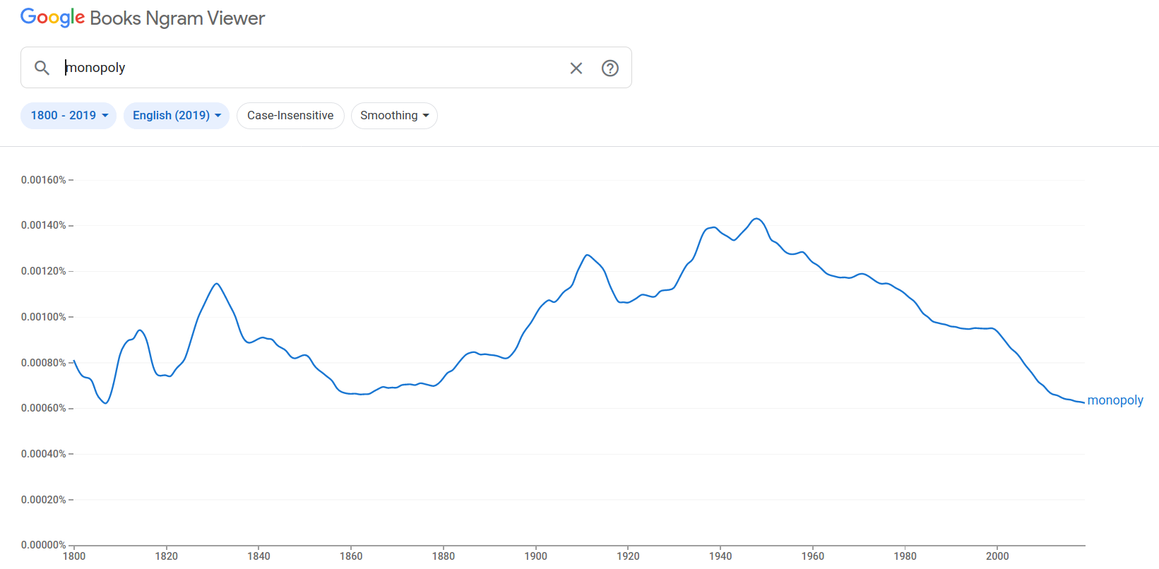 Pretty cool, right?
Downloading the data
You’ve found some data that looks interesting. The next step is to download it onto your computer so you can work with it. Often, this is as simple as clicking Download. But in the case of the Ngram Viewer, this option isn’t available. (Look for yourself. The  button in the top right corner looks promising. It has an option to
 Download raw data. But that doesn’t download the data on your graph. It takes you to the bulk repository for the Ngram database, which we’ll discuss shortly.)
Although there’s no Download button, you can still download data from the Ngram Viewer. But you’ll have to do some hacking. Software developer Johannes Filter walks you through the steps here. Basically, you get the data you want on the screen. Then you open your web browser’s developer tools and look at the page’s source code. From there, you copy and paste the ngram data into a text file where you can work with it. (Note: the Ngram viewer automatically smooths the data. For empirical work, you want the unsmoothed data. Get this by setting Smoothing to 0.)
This browser hack isn’t pretty, but it works. If you want data for one or two words, this hack is probably the fastest method. (It’s how I got the data for free-market speak analyzed here). That said, if you want data for more than a few words, the browser hack is too clunky.
Using R packages
I love R. If you’re not familiar, R is a programming language for statistical computing. Over the years, it’s evolved into a huge ecosystem of tools for doing analysis. If there’s empirical work you want to do, chances are there’s an R package for it. In the case of the Google Ngram dataset, there’s a convenient R package called ngramr.
Before we dive into the ngramr package, let’s talk about when/why you should use software packages to get data. To use a package, you have to spend time learning its syntax. If you’re doing a one-off analysis, you probably don’t want to invest this time. But if you’re getting data repeatedly, it’s worth your time to learn how to use a dedicated package.
Back to the R ngramr package. In this case, the syntax is simple. The package provides a function called ngram() that retrieves data from Google. To get data for the word ‘monopoly’, you’d enter:
ngram("monopoly")It will return a data frame with the relative frequency of the word ‘monopoly’ in different years:
  Year   Phrase    Frequency   Corpus
1 1800 monopoly 8.104906e-06 eng_2019
2 1801 monopoly 7.628060e-06 eng_2019
3 1802 monopoly 7.339290e-06 eng_2019
4 1803 monopoly 7.332237e-06 eng_2019
5 1804 monopoly 7.272125e-06 eng_2019
6 1805 monopoly 6.520742e-06 eng_2019
# … with 214 more rows
That’s easy! Now suppose you want to look up data for several words. Still easy. The ngram() function can take a ‘vector’ input (i.e. a list). To use this feature, first bind the words you want in a vector using R’s c() function. Then dump that vector into the ngram function. Suppose we want data for the words ‘monopoly’, ‘demand’ and ‘price’. First, bind the words into a vector:
words = c("monoploy", "demand", "price")Then throw that vector into the ngram function:
ngram(words)Perhaps you only want data starting in 2018. No problem. Just specify the start year:
ngram(words, year_start = 2018)Here’s the result:
  Year   Phrase    Frequency   Corpus
1 2018 monoploy 3.376117e-10 eng_2019
2 2019 monoploy 3.376117e-10 eng_2019
3 2018   demand 5.667883e-05 eng_2019
4 2019   demand 5.667883e-05 eng_2019
5 2018    price 7.255132e-05 eng_2019
6 2019    price 7.255132e-05 eng_2019
As you can see, the ngramr package is easy to use. If you want Ngram data for a few hundred words (or even a few thousand), this package is your best bet.
Scaling up
A rule of thumb for empirical work is that your method will depend on how much data you’re analyzing. Let’s use the Ngram data to illustrate.
If you want data for one or two words, the fastest approach is probably the browser hack. If you want data for hundreds of words, your best bet is the ngramr package. But what if you want data for hundreds of thousands of words? Then you need a different approach.
The problem with the ngramr package is that it’s ‘slow’. I’ve used scare quotes here because you have to take the word ‘slow’ in context. The ngram() function limits you to retrieving data for 12 words at a time. So if you want data for hundreds of words, you’ll have to make a loop and use the ngram() function multiple times.
That’s no big deal. However, the main limitation is that ngram() takes about 1 second to get data for 12 words. If you want data for a few hundred words, it will take a few minutes of computation. That’s not bad. But if you want data for 500,000 words, you’re looking at more than 11 hours of computation. That’s too slow for my taste.
The reason ngram() is slow, it turns out, is because it’s actually an automated version of the browser hack I discussed above. Under the hood, ngram() goes to the Ngram Viewer website, searches for the words you want, and then scrapes the data from the html. That’s pretty clever. But it’s also slow.
Back to empirical work in general. A rule of thumb is that tools that are convenient for small-scale analysis don’t work when you move to the large scale. When you want to analyze big data, you need to do a bulk download.
Bulk downloads
When you’re doing large-scale analysis, bulk download centers are your friend. They allow you to download an entire dataset in one go. That’s helpful when you want to analyze a lot of data.
Here’s an example. A few years ago, I analyzed the price change of every commodity on the consumer price index (CPI). (See the results here). That would have been unthinkable if I had to download each price series individually. Instead, I bulk downloaded the entire CPI dataset here.
Bulk downloads, however, come with a cost. They’re usually frighteningly opaque. Unlike with small-scale data, bulk downloads generally don’t describe the data. Instead, you’ll see a bunch of codes. Here, for example, is the bulk data for the consumer price index. There’s nothing but numbers and codes.
The cost of using bulk downloads is that you have to spend time figuring out how the dataset is coded. You do this using a codebook. (Here’s the CPI codebook.) The problem is that codebooks are usually written by statisticians who already know the data well. For the novice analyst, codebooks can be as opaque as the raw data. I’ve spent many frustrating hours trying to decipher a database’s codebook.
Back to the Ngram data. The bulk download center for the Google Ngram data lives here:
http://storage.googleapis.com/books/ngrams/books/datasetsv3.html
Unlike with the Ngram viewer, here there are no graphics, no search bars, and no buttons. There’s just text and hyperlinks. It’s up to you to figure out what to do.
After using the data for a few months, here’s what I’ve learned. First, there are three different versions of the Ngram dataset:
- Version 1 (created in 2009)
- Version 2 (created in 2012)
- Version 3 (created in 2020)
Second, the entire datasets are unmanagably huge. So you’ll have to work with a subset of the data. For me, that means downloading only the ‘1-gram’ data (text frequency for single words).
Third, each version of the database is structured differently. In short, when you start working with the raw Ngram data, you’re opening a can of worms.
The 2012 Ngram corpus
Let’s start with the 2012 corpus, because it’s the easiest to work with. The data comes in compressed text files. When you unpack them, each file will contain something like this:
circumvallate   1978   335    91
circumvallate   1979   261    91
(+ 50 million more lines)
As is typical with bulk downloads, there’s no labels. It’s up to you to figure out what the data means. It turns out that the first column is the ngram. The second column is the year. The third column is the number of times the ngram occurs. And the fourth column is the number of ‘volumes’ (i.e. books) in which the ngram is observed.
Alright, we’ve figured out what the data means. Now how do we work with it? To work with data, we usually read the whole dataset into the computer’s memory. But with the Ngram data, that’s not an option. The 2012 1-gram dataset is about 24 GB. Even if your computer has that much RAM, you’d need even more if you want to manipulate the data. So reading the whole dataset into memory is probably not going to work.
So what should we do? The solution is to do our analysis in pieces. The 2012 1-gram dataset comes in 26 different files — one for each letter of the alphabet. Each file is about 1 GB, which can easily fit into your computer’s memory (unless you’re using something ancient). So here’s the approach. You read each file into memory. Then you look for the words that you want. You keep the data for these words and discard the rest. Then you move on to the next Ngram file. Repeat.
Data formats
Alright, we’re caught up to where I was two weeks ago. I’d first retrieved ngram data using the browser hack. Then I’d run some analysis with the ngramr package. After realizing that this was going to be too slow, I downloaded and analyzed the 2012 1-gram dataset. I was writing up my results when … I discovered that there was a 2020 Ngram dataset.
No big problem, you’d think. Just download the new data and rerun your analysis. If only it were that simple. The problem, I discovered, was that the 2020 Ngram data comes in a completely different format — one that is not easy to use.
To understand the problem, let’s talk data formats. Big datasets are usually stored as plain text. That means if you open up the file with a text browser, you’ll see a bunch of text. As I’ve already discussed, the 2012 Ngram data looks like this:
word            year   count  volume
circumvallate   1978   335    91
circumvallate   1979   261    91
This is called ‘tab separated data’. Within each line, the different entries are separated by a TAB. Another common approach is to separate data by commas, like this:
word,year,count,volume
circumvallate,1978,335,91
circumvallate,1979,261,91
The comma-separated approach is a bit harder for humans to look at. But for your computer, it’s easy to read. In principle, data can be separated (‘delimited’) by any character. But commas and tabs are the most common.
What’s most important here is not the data-separating character, but the fact that the 2012 Ngram data is ‘rectangular’. Each line has the same number of entries. In other words, the data has a fixed number of columns.
This is important because most data-reading tools work best when the data is rectangular. Let’s use R as an example. In R, there’s a whole ecosystem for reading rectangular data. In ‘base R’, there’s read.csv(), which parses comma-separated files. For tab-separated data, there’s read.table(). These functions will read the data and format it into an easily-manipulable data frame.
For big datasets, these base functions are a bit slow. If you want speed, I recommend the fread() function from the data.table package. There’s also a family of functions available in the readr package.
What all of these functions have in common is that they’re built for parsing rectangular data. If your data comes in some other format, you’re out of luck. That brings me to the 2020 Ngram corpus.
The 2020 Ngram corpus
Unlike the 2012 corpus, the 2020 Ngram corpus is not stored in a ‘rectangular’ format. Instead, the data looks like this:
ngram               Year,count,volume   Year,count,volume   …
Breadberry          1785,1,1            1795,1,1            …
byzantinological    1962,2,2            1976,1,1            …
Here, each ngram gets its own line. Year, count and volume information then follow, separated first by a TAB, and then by commas. What’s important is that the number of entries in each line varies by ngram. (Some ngrams have data covering only a few years. Others have data covering hundreds of years.) In other words, the 2020 Ngram data is not rectangular. So standard data-reading functions won’t work.
Why the odd formatting? My guess is that Google used it to save space. In the rectangular format, notice that each ngram gets repeated for each different year in which it occurs. In the new format, each ngram appears once. When you have billions of ngrams, that saves a lot of space. Still, the 2020 1-gram corpus is huge — about 44 GB. So we need a way to parse the data fast and efficiently.
Let’s pause here and talk about a trade off in data analysis (or any software development, for that matter). There’s always a trade off between computation time and programmer time. If you want code that executes quickly, it will take more time to program. If you want code that’s written quickly, it will execute more slowly.
A good rule of thumb is that your time is more important than your computer’s time. (Remember that you can do other things while your computer crunches numbers.) If you spend 10 hours writing code that saves the computer 10 seconds, you’re wasting your time. But if 10 minutes of coding will save 10 hours of computation, that’s worth your while.
Back to the Ngram data. In R, there’s a base function called readLines() that does what it says — it takes lines from a file and reads them into memory. What’s useful about this function is that it’s form agnostic. It doesn’t care if the data is rectangular. The cost, however, is that the data gets returned in a way that’s not very usable. You’ll get a character vector, where each element contains the characters on a given line. When read with readLines(), the 2020 Ngram data would look like this (\t is computer code for TAB):
"Breadberry\t1785,1,1\t1795,1,1…", "byzantinological\t1962,2,2\t1976,1,1…"This is ugly. Yes, the data is in your computer’s memory. But without more cleaning and processing, the data is useless. So the question is, how do you want to clean it?
Answering this question depends on how much data you have. In a file with a few hundred lines, I’d use R to read and clean the data. The code would take me a half hour to write and would execute in milliseconds. The Google Ngram data, however, has billions of lines to read and clean. Doing that in R won’t take milliseconds. It could take hours.
If I’m going to run the code once, that’s not so bad. I press ENTER, let the code run, and write some emails for an hour. The problem, though, is that empirical analysis almost never gets done once. You inevitably find mistakes, get new ideas, or expand your analysis. And so you rerun the code. That 1 hour run-time just to read and clean the data quickly becomes frustrating.
If you’re going to run analysis many times, it’s probably worth it to write faster code. For me, that means turning to the programming language C++. Unlike R, which is an ‘interpreted language’, C++ is a ‘compiled’ language. That makes it much faster (to execute, not to code).
One of the things I love about R is that it’s easy to integrate with C++. There’s a package called Rcpp that lets you write C++ code and import it seamlessly into R. Whenever I want speed, this is my go-to method.
Back to the Ngram data. To crunch the 2020 data, I ended up writing two C++ functions. (The code lives here.) The first function is called get_ngrams(). As it suggests, this function parses an Ngram 2020 file and returns a list of all the ngrams in it. Run the function like this:
ngrams = get_ngrams("ngram_file")The get_ngrams() function is useful because in most cases, we’re interested in only a tiny subset of the ngrams in the Ngram file. So we don’t want to waste time parsing all of the data. Instead, we run get_ngrams(), which will take a few seconds to execute. Then we have a list of the ngrams in the file.
The next step is to select the ngrams we want, and get data for them. In my case, I’m interested in the ngrams that are actual English words. As an example, let’s get data for all of the ngrams that are in the grady_augmented word list (a list provide by the R lexicon package). The code would look like this
ngrams = get_ngrams("ngram_file")
ids = which(ngrams %in% lexicon::grady_augmented)
ngram_data = get_data("ngram_file", ids)
Here’s what the code does. First we get a list of all the ngrams in the file. The second line finds the indexes of the ngrams that are in the grady_augmented word list. The third line gets data for these ngrams.
This code allows me to extract data for hundreds of thousands of ngrams in about 5 seconds. That’s fast. With this code, I can parse and analyze the whole 2020 1-gram database in about 5 minutes. So when I inevitably rerun the analysis, I won’t have to wait long. (Just enough time to make a coffee.)
That said, it took me a few days to write the C++ code. That’s because I took several wrong turns along the way. Did I waste my time? Perhaps. But I like to consider three factors besides raw time. First, I enjoy coding in C++ (I always learn something new). Second, I plan on using this code many times in the future. Third, I’m sharing my code (here). That means I’m not just saving my time. I’m potentially helping other researchers save time.
How deep do you want to go?
Alright, let’s wrap up this foray into Ngram analysis. If you’re a researcher who’s interested in Ngram data, I hope the above information is useful.
That said, I know that the majority of readers aren’t Ngram researchers. Still, there are general principles that are useful. When you do empirical work, the deeper you go, the harder it gets. If you want to do exploratory analysis, it’s usually simple. Dump some data in a spreadsheet and plot it. But if you want to go deeper, it will take more time. You’ll probably have to use a new package. And if you want to go deeper still, you may have to write custom code.
At each step, you need to think before you dive in. Do you want to pay the costs of going deeper? The reward is better analysis. The cost is time … and lot’s of it.
And that brings me to the third reason for telling you about my foray into Ngram analysis. When I finally (hopefully next week) show you my results for relative word frequency in economics textbooks, I want you to know how much damn work it took.