The Deep History of Human Inequality

In his epic 18th-century treatise Discourse on Inequality, Jean-Jacques Rousseau argued that inequality is an ill of civilization, created by private property. If you roll back the clock on civilization, he claimed, you should also roll back inequality.

Rousseau was probably both right and wrong.

He was right in the sense that civilization does seem to produce inequality. But Rousseau was wrong in the sense that prior to civilization, he envisioned a static ‘state of nature’ in which humans lived in harmony. In other words, Rousseau knew nothing about human evolution. But today we do.

In this post, I look at the evidence for inequality in our evolutionary past. The evidence hints, I argue, that our ancient ancestors were quite different than the hunter-gatherers of today. Rather than be fiercely egalitarian, our ancestors may have lived with significant inequality. No, they didn’t squabble over mansions and mutual funds, as we do now. They squabbled over sexual mates. Or at least the males likely did.

Today, humans are a species that biologists would call ‘mildly polygynous’. That means it is not uncommon for a man to have multiple mates simultaneously. (A linguistic note: We often call this practice ‘polygamy’, but the more precise word for males (but not females) having multiple partners is ‘polygyny’.) True, polygyny is becoming less common in many parts of the world. But that may be a recent trend. In our deep past, humanity may have been far more polygynous. And that means the sex life of ancestral males would have been more unequal.

Of course, we cannot observe this ancient sex life directly. But we may be able to observe it indirectly … by looking at body proportions. Today, men are slightly larger than women. This is a form of what biologists call ‘sexual dimorphism’ — a difference between sexes that goes beyond having different reproductive organs. It turns out that among primates, sexual size dimorphism correlates with polygyny. The more polygynous the species, the more that males tend to outsize females.

When we map this correlation onto our evolutionary history, we find something startling. Contrary to what Rousseau thought, humans may not have a deep history of egalitarianism. Instead, our dominant male ancestors may have been remarkably despotic. If this is true, it means that human egalitarianism may be a recent adaptation — so recent that the driving force may not have been our genes, but rather, our culture.

Rolling back civilization’s clock

Let’s start our foray into the deep history of inequality by looking at what Rousseau got right. As we roll back civilization’s clock, inequality tends to disappear.

Figure 1 shows the trend, which is part fact, part speculation. The factual part is the data within the last 10,000 years. The black points are estimates of the inequality found in various Old-World archaeological sites. The blue curve shows the smoothed trend, which is clearly upward. As civilization emerged, inequality tended to increase.

The speculative part of Figure 1 is what came before the archaeological record. Today, we observe that hunter-gatherer societies (like the !Kung of Africa) have little inequality. If our ancestors lived like these societies do now, then human prehistory would have been marked by low inequality. Figure 1 shows what this might have looked like.

Not everyone agrees with this type of inference. In a recent article, anthropologist David Graeber and archaeologist David Wengrow warn against projecting the behavior of modern hunter gatherers into the distant past. Doing so, they argue, evokes the “eternal return of Jean-Jacques Rousseau”. The tale invented by Rousseau is that inequality emerged with agriculture. The problem, Graeber and Wengrow observe, is that this is factually wrong. The evidence for inequality long predates formal methods of farming.

I’ll grant Graeber and Wengrow this evidence, but doubt that it changes the big picture of inequality. There seems little question that rampant despotism is a recent invention, and that in our prehistory there was far less inequality. What remains unknown is the exact timing of the transition. Was it recent and sharp, as depicted in Figure 1? Or was it deeper and smoother?

These are important questions, but ones that I won’t address here. Instead, I’m interested in the red line in Figure 1 — a line that I’m calling ‘Rousseau’s boundary’. In our distant past, Rousseau imagined that humans lived in a ‘state of nature’. It was a state that, for all he knew, continued indefinitely back in time. Today, we know this is untrue.

Like all species, humans evolved. So over evolutionary time, our behavior has been in constant flux. The question is how? As we cross Rousseau’s boundary, what happens to ‘human’ inequality? (I use scare quotes here, because the farther back we go, the less ‘human’ we become.)

For the rest of the post, I try to piece together the evidence.

Crossing Rousseau’s boundary

I’ll begin the journey beyond Rousseau’s boundary by giving some credit. Until recently, I’d never thought about what inequality was like in humanity’s evolutionary past. I took Rousseau’s ‘state of nature’ as a given — something I didn’t think beyond. In hindsight, that was foolish.

Today, I know there is a rich literature that speculates about how our ancient ancestors might have behaved. Much of the evidence suggests that we were once quite different — more sexually dimorphic and hence likely more unequal in the way we practiced mating. But as an economist (not an anthropologist), I was blissfully unaware of this research.

Fortunately, biologist (turned social scientist) Peter Turchin relieved me of my ignorance. In a blog post called ‘The Z-Curve of Human Egalitarianism’, Turchin speculates about the deep history of human inequality. If our primate relatives are any indication, Turchin notes, our ancient ancestors may have been rather despotic:

We know that our closest relatives, the chimps and gorillas, live in fairly ‘despotic’ or inegalitarian societies. The chimps, for example, establish linear dominance hierarchies, in which alpha males get better food and greater access to females. We don’t know for sure whether human ancestors also lived in similarly inegalitarian societies, but it seems likely.

(Peter Turchin, 2012)

Looking at our primate cousins, Turchin infers that human evolution has a ‘U-shaped curve of despotism’. As we split from gorillas and chimps, inequality declined, only to re-emerge later with civilization. Turchin leaves this deep history as a qualitative speculation. But I’m going to try to make things quantitative. The way I’ll do it is by looking at body size.

Sexual dimorphism as a window into polygyny

That men tend to be larger than women is obvious. What is less obvious is that this size difference tells us something about behavior. But it likely does. In primates (and other mammals), the size difference between males and females seems to be connected to ‘polygyny’ — the practice of males having more than one mate.

Before we dive into this connection, let’s first review some basics about biology. The size difference between men and women is part of a larger suite of physical differences that biologists call ‘sexual dimorphism’. These are differences between sexes that are not directly related to reproduction.

Sexual dimorphism is ubiquitous, but varies greatly between species. In birds, males are usually more colorful than females, and tend to have more elaborate plumage. In primates, sexual dimorphism usually takes the form of a size difference. Males are usually larger than females. But how much larger depends on the species.

In humans, size dimorphism is modest. The average man is about 15% heavier than the average woman. Although that difference may appear significant, it’s a small degree of dimorphism compared to what we find among our primate relatives. Take gorillas. Male gorillas typically outweigh females by 90%. If we map that difference onto humans, the average American man would weigh about about 315 pounds.¹ In reality, few men achieve this weight. (And when they do it’s usually from obesity.) So gorillas are far more sexually dimorphic than humans, something that is obvious when you compare the two species.

It turns out that among primates, humans are at the lower end of the dimorphism spectrum. Figure 3 illustrates this fact. I’ve plotted here the distribution of sexual size dimorphism among primate species. The horizontal axis shows the ratio of male-to-female weight within a species — what I will call the ‘degree of sexual dimorphism’. The vertical axis shows the number of species with the given level of dimorphism. Across all species, primate males are on average about 35% heavier than females. So the 15% mass difference between men and women is at the lower end of the primate spectrum.²

Among primates, sexual size dimorphism is ubiquitous. The question is, why? If you’re stumped by this question, don’t worry. You’re in good company. For a decade, the question of sexual dimorphism stumped none other than Charles Darwin.

In 1859, Darwin published his theory of natural selection, which proposed that organisms evolve adaptations that are useful for survival. He was driven to this idea because useful adaptations are everywhere (i.e. eyes, wings, legs, teeth, etc.). Yet upon further reflection, Darwin noticed that some traits — especially non-reproductive differences between sexes — appear useless, or even burdensome. What kept Darwin up at night was the peacock’s tail. It was massive, elaborate, and seemingly purposeless. Darwin complained:

The sight of a feather in a peacock’s tail, whenever I gaze at it, makes me sick!

(Charles Darwin, 1860)

After thinking about the problem of sexual dimorphism for a decade, Darwin discovered a solution. Evolution was not just about survival of the fittest. It was also about the fit reproducing. And to reproduce, you had to win a mate.

Darwin realized that the competition for mates could cause weird traits to evolve — traits that had little to do with survival. For instance, if members of one sex developed certain mating preferences, that would put pressure on the opposite sex to evolve the desired traits. It didn’t matter if the traits benefited survival. As long as they benefited mating, traits that were seemingly detrimental could still evolve.

Darwin called this process ‘sexual selection’, and proposed that it explained the peacock’s tail. The purpose of the male’s tail, Darwin argued, was solely to impress females. Sure, the preposterous tail got some males killed. But since females desired the elaborate plumage, males without it would be perpetual bachelors. And in evolutionary terms, that’s the same as being dead.

So sexual selection, Darwin argued, explains the evolution of sexual dimorphism. Still, questions remained. Why, for instance, was the peacock’s elaborate tail a feature of the male? Why not the female? Darwin thought this wasn’t a coincidence. That’s because across species, it is almost always males that are modified by sexual selection:

Throughout the animal kingdom, when the sexes differ in external appearance, it is, with rare exceptions, the male which has been the more modified; for, generally, the female retains a closer resemblance to the young of her own species, and to other adult members of the same group.

(Charles Darwin, 1871)

The reason that males are more modified, Darwin proposed, is that they are subject to more intense sexual selection. That’s because the male’s role in reproduction is different than the role of the female. Females gestate offspring. Males contribute nothing but sperm. That means winning many mates affects males and females differently. No matter how many mates a female wins, her reproduction is limited by the need to gestate offspring. Not so for males. The more mates a male wins, the more offspring he produces.

This asymmetry means that the mating stakes are higher for males. If a male loses the mating game, he will have no offspring — just like a losing female. But unlike a female, when a male wins the mating game, he can win big. A male with a large harem can produce hundreds (even thousands) of heirs. This potential to win big puts more selective pressure on males to develop what Darwin called ‘secondary sexual characters’ — traits that differ between sexes but are not used directly for reproduction.

In birds, sexual selection caused males to evolve elaborate plumage. In primates, it caused males to grow larger than females. And because humans are primates, Darwin realized that the same principle applies to size differences between men and women. Men are larger than women because of the competition to win mates:

There can be little doubt that the greater size and strength of man, in comparison with woman, [is] due in chief part to inheritance … by the success of the strongest and boldest men, both in the general struggle for life and in their contests for wives …

(Charles Darwin, 1871)

So according to Darwin, sexual selection explains both the existence of sexual dimorphism and why it is usually males that are more modified. But what explains the differing degrees of dimorphism between species? Again, Darwin had an answer. Variation in dimorphism was caused by variation in polygyny:

That some relation exists between polygamy and the development of secondary sexual characters, appears nearly certain …

(Charles Darwin, 1871)

Polygyny, as a reminder, is the practice of males having multiple mates. (The word ‘polygamy’, used by Darwin, is more common, but technically refers to any multi-partner arrangement.) Darwin noticed that in species that were more polygynous, sexual dimorphism was more extreme. Why?

The answer is that the ‘degree of polygyny’ affects the reproductive stakes. In a monogamous species, most males will win a mate. So sexual selection pressure is low, and there is little reason for males to differentiate themselves. But if a species is highly polygynous, the winning males can vastly out-reproduce the losers. These high stakes put intense pressure on males to develop secondary sexual characteristics. And so they do.

As an example of the extremes of both polygyny and sexual dimorphism, consider the elephant seal. Male seals compete violently for females, with the winner acquiring a huge harem. As a result, dominant bulls vastly out-reproduce the losers. One study found that 4% of males inseminate 85% of females. This implies that the top males outbreed the losers by a factor of 130.³ With such high stakes, there is intense selective pressure on males. The evolutionary response has been for male elephant seals to get big … absurdly big. A large bull can outweigh a female by a factor of 10.

Among primates, polygyny and sexual dimorphism are less extreme, but still related. Figure 4 shows the data. The horizontal axis shows the degree of sexual dimorphism within a species. The vertical axis shows the ‘degree of polygyny’ — the average number of females per reproductive male.

The correlation between polygyny and dimorphism isn’t perfect, but it’s enough to make rough predictions. Judging by our sexual dimorphism, humans evolved as a slightly polygynous species. If we feed our degree of dimorphism into the primate trend, I predict that humans have a degree of polygyny (average harem size) of about 1.5.

Keep in mind that this is not a prediction for how humans behave now, but rather, a prediction for how we behaved in the past. Our dimorphism suggests that in our recent evolutionary past, humans were a mildly polygynous species. Of course the word ‘mild’ needs context. A degree of polygyny of 1.5 implies that many reproductive males had two mates. Compared to other primates, that’s ‘mild’ polygyny. But it’s enough polygyny to make many ‘civilized’ humans uncomfortable.

Polygyny as inequality

Why care about polygyny? Because it is the principle form of inequality in the animal world.

That this is true, though, is not immediately obvious. In polygynous species, it could be that females outnumber males. If they did so in proportion to the degree of polygyny, then all males could have an equal number of mates. Polygynous mating would therefore be ‘fair’ (for males).

In practice, this fairness does not occur. That’s because polygyny does not come with a corresponding abundance of females. Instead, most species have a balanced sex ratio, regardless of their degree of polygyny. This fact, known as ‘Fisher’s principle’, is one of the most celebrated regularities in biology. It occurs because a one-to-one sex ratio is the only evolutionarily stable strategy. If one sex grows over-represented, it becomes advantageous to produce the under-represented sex. The result is a pendulum oscillation around a one-to-one sex ratio. Richard Dawkins explains:

Suppose that … a mutant gene arose that tended to make parents have mostly daughters. … But now, think what an enormous genetic advantage is enjoyed by those few parents who have sons. … Therefore genes for producing sons will tend to become more numerous, and the pendulum will swing back.

(Richard Dawkins, 1976)

Because it is the only stable strategy, virtually all species have a one-to-one sex ratio. As such, when species practice polygyny, male reproductive success is automatically unequal. So we can think of polygyny as the forced production of bachelors. Psychologist David Barash elaborates:

[In a polygynous species] a small number of males get to father many offspring, whereas most males are reproductive losers, ending up as unmated, frustrated, and resentful bachelors. The greater the “degree of polygyny” … the more bachelors.

(David Barash, 2016)

With bachelors in mind, let’s talk numbers. We can quantify the production of bachelors the same way we quantify any form of inequality — using the Gini index. We take the distribution of harem size (the number of females per reproductive male) and plug it into the Gini formula. The result is a measure of male reproductive inequality.

That’s simple enough … except there’s a catch. The required data (the distribution of harem size) is usually not available. Fortunately, this data is easy to simulate. If a species has equal numbers of both sexes, then we can estimate male reproductive inequality from the degree of polygyny. Figure 5 shows my estimate. (Technical details are here.)

As the degree of polygyny grows, male reproductive inequality explodes. Along the curve in Figure 5, I’ve labelled various primate species based on their observed degree of polygyny. Species that are monogamous, like the three-striped night money, have virtually no reproductive inequality. But as polygyny increases, reproductive inequality grows. In highly polygynous species, like the patas monkey, male reproductive inequality is extreme.

The red region in Figure 5 shows where humans likely sit. I’ve estimated human polygyny from our level of sexual dimorphism (Fig. 4). As a slightly polygynous species, I peg the reproductive inequality of ancestral human males at a Gini of 0.5 \pm 0.1.

Having equated polygyny with ‘inequality’, it’s worth mentioning that biologists usually adopt language that is more neutral. They say that polygyny affects ‘variance’ in male reproductive success. The reason for this neutral language is that biologists want to avoid value judgments about other species. That’s why when one animal kills another, biologists don’t call it ‘murder’. Nor do they call violent mating ‘rape’. These words reflect human taboos. But nature, as far as we can tell, has no moral boundaries.

I’ve decided to use moralizing language, however, because I’m explicitly interested in the history of human behavior. On that front, humans seem to have a deep-seated aversion to inequality. The surest way to evoke human outrage is to claim that someone took more than their fair share.⁴

Have humans always valued equality? The fact that men are larger than women suggests that we evolved as a mildly polygynous species. So our recent male ancestors tolerated modest sexual inequality. But what were we like in the deep past? Judging by our primate relatives, our ancient ancestors may have been far more tolerant of despotism.

Humanity’s evolutionary tree

I’m going to use our evolutionary tree to infer rates of (sexual) inequality in our deep past. The first step, then, is to define humanity’s family tree.

In a recent paper, Luca Pozzi and colleagues used DNA to infer both the structure of our evolutionary tree and the timing of the various branches. Figure 6 shows their results. It’s a remarkable piece of science.

Primates first evolved some 80 million years ago. At the time, our distant ancestors were a niche species in a landscape dominated by dinosaurs. That changed 65 million years ago when a mass extinction killed off the dinosaurs, along with many other species. Our primate ancestors survived this crisis, after which they ‘radiated’ into many ecological niches. The evolutionary story is long, fascinating, and still poorly understood.

What I’ll focus on in Figure 6 are the nodes of the evolutionary tree. Each node represents a common ancestor of two related species. Let’s look at the Homo sapiens lineage. Node 1 is the common ancestor of humans and Neanderthals. Node 4 is the common ancestor of humans and chimps. Node 5 is the common ancestor of humans and Gorillas. As we go farther back in time, we eventually reach node 61, the common ancestor of all primates.

With humanity’s lineage in mind, let’s take a guess at what our ancient ancestors were like.

The deep history of ‘human’ sexual dimorphism

I’m going to use the evolutionary tree in Figure 6 to estimate the degree of sexual dimorphism in our ancient ancestors. Here’s the method. I start with living primates whose sexual dimorphism we know. I then move backwards on the evolutionary tree, using the traits of descendants to estimate the traits of their common ancestor. Each time a branch merges (going back in time), I estimate the sexual dimorphism of the common ancestor by averaging the dimorphism of the descendants.

Here’s an example. About 700,000 years ago, humans shared a common ancestor with Neanderthals (node 1 in Fig. 6). I estimate this ancestor’s sexual dimorphism by averaging the dimorphism of the two descendents: humans (dimorphism = 15%) and Neanderthals (dimorphism \approx 17%). That puts the dimorphism of the ‘sapiens-neanderthals’ ancestor at about 16%.

Let’s go back further. About 7 million years ago we reach node 7 — the common ancestor of humans (the homo genus) and chimps (the pan genus). Today, chimp males are about 30% heavier than females. Averaging that value with the 17% dimorphism of the ‘sapiens-neanderthals’ ancestor gives a sexual dimorphism for this ‘homo-pan’ ancestor of 23%.

We can keep going like this until we’ve traversed the entire evolutionary tree. The result is an estimate of the sexual dimorphism of every ancestral node in Figure 6. With this estimate in hand, we can infer the evolution of dimorphism in our ancient ancestors.

Figure 7 shows the results. Here each point represents a common ancestor of the human lineage. I’ve labelled these ancestors by the primate taxa being ‘merged’, the taxonomic rank of the merger, and the corresponding evolutionary node in Figure 6. Here’s an example. The point labelled ‘Hominini-Gorillini’ represents the common ancestor of humans and gorillas. It occurs at node 7 (in Fig. 6) and represents the common ancestor of living taxa at the ‘tribe’ level.

Today, human males are only slightly larger than females. But the evidence suggests that this has not always been so. Our closest living relatives — chimps and gorillas — have far more sexual dimorphism than us. If our common ancestors were somewhere in the middle (as I’ve assumed), then they must have been more dimorphic. Figure 7 shows how this might have evolved. Moving backwards in time, ancestral dimorphism may have increased all the way back to our common ancestor with orangutans (‘Homininae-Pongo’). Going back further, dimorphism may have then declined. The caveat, of course, is that the further back we go, the more uncertain is our inference.

That our ancestors had greater sexual dimorphism is also supported by the fossil record. The red points in Figure 7 show dimorphism estimates for extinct species of hominid. Interestingly, the fossil record indicates that dimorphism changes may have come recently, not long before our shared ancestor with Neanderthals.

While the uncertainties are large, the evidence suggests that our ancient ancestors were more sexually dimorphic than us. This hints that they may have also been more despotic.

The deep history of male reproductive inequality

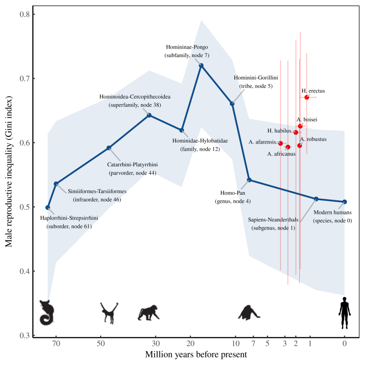
With our sexual dimorphism estimates in hand, let’s go one step further and estimate the deep history of male reproductive inequality. Figure 8 shows what this evolution might look like. (Methods details are here.)

The results suggest that after we parted ways with gorillas, male reproductive inequality trended downward. What’s uncertain, however, is the timing of this trend. My phylo-based estimate (blue) suggests that male reproductive inequality decreased slowly as we split from gorillas and chimps. But the fossil record (red) suggests that the shift came later, and more rapidly. Extinct hominids who lived just before our Sapiens-Neanderthals ancestor seem to have had far more reproductive inequality than modern humans (or so we infer).

Is egalitarianism a cultural adaptation?

Let’s assume that our ancient ancestors were more polygynous (and hence, sexually unequal) than we are today. The question is — how did we evolve to be egalitarian?

There’s no question that the evolution was in part genetic, since the shift is written on our bodies (as decreasing sexual dimorphism). But that doesn’t mean culture was unimportant. My guess is that the evolution of egalitarianism was shaped by both genes and culture.

Here’s a possible route. Polygyny involves the forced production of bachelors, who are evolutionary losers. These bachelors are usually smaller and weaker than the dominant males, which is why they can’t win mates. But here’s the thing about polygyny: there are always more bachelors than there are dominant males. So why don’t these bachelors gang up on the big males to knock them down a peg?

Well, it turns out that one species of primate does just that. And that species is … us. The anthropologist Christopher Boehm calls this human behavior ‘reverse dominance’. In hunter-gatherer societies, when an individual accumulates too much power, subordinates gang up on the would-be ruler. The effect of this reverse dominance, Boehm argues, is to maintain equality.

It seems plausible that this cultural behavior shaped our genetic evolution (and vice versa). If our ancestors practiced reverse dominance, that would tend to suppress polygyny. And suppressing polygyny would in turn ease selective pressure on males, causing sexual dimorphism to decrease. That would make reverse dominance easier, causing the whole loop to feed back on itself: culture \longrightarrow genes \longrightarrow culture \longrightarrow genes …

Going further, it could be that culture was essential for reversing polygyny. That’s because practising reverse dominance requires collective action. It’s only by working together that bachelors can depose the big boys. So it seems plausible that without cultural tools like language, reverse dominance would have been impossible.

This is all speculation, of course. But as a rule of thumb, the faster a behavioral change occurs, the more likely that culture (not genes) is at play. On that front, the reproductive inequality of our male ancestors may have dropped in an evolutionary blink of the eye. Extinct species like Homo erectus seem to have been highly polygynous. Yet our Sapiens-Neanderthal ancestor, who lived not long after, was more monogamous (we infer). This is a tantalizing hint that the evolution of egalitarianism may have been shaped by the evolution of culture.

---

---

Sources and methods

Inequality data in Figure 1 is from Kohler et al. (2017).

Sexual dimorphism and polygyny data

• Cassini (2020), primate dimorphism and polygyny
• Clutton-Brock et al. (1977), primate dimorphism and polygyny
• Froehle and Churchill (2009), Neanderthal dimorphism
• Kappeler (1991), primate dimorphism
• Larsen (2003), human dimorphism
• Leigh (1992), primate dimorphism
• McHenry (1994), dimorphism in extinct hominids
• Mitani et al. (1996), primate dimorphism and polygyny

Model of male reproductive inequality

Here’s how I estimate the Gini index of male reproductive inequality as it relates to the degree of polygyny. I assume that (adult) male mating success is lognormally distributed. The number of females f_m with which a male mates is a lognormal random variate:

Here N_m is the number of males, \mu and \sigma are lognormal parameters, and \left\lfloor\right\rfloor denotes rounding down to the nearest integer.

The degree of polygyny, DP, is defined as the average number of females per male who is sexually active (has more than 0 mates):

I assume that all adult females are sexually active, which means the adult female population is the sum of f_m across all males:

I restrict the parameter space \left\lbrace \mu, \sigma \right\rbrace to that which produces a sex ratio within 1% of one-to-one:

For any given parameter combination (\mu, \sigma) , male reproductive inequality MRI is the Gini index of the variate f_m :

When we iterate over the parameter space \left\lbrace \mu, \sigma \right\rbrace , sampling distributions of f_m , we get a numerical relation between the degree of polygyny DP and male reproductive inequality MRI.

Some caveats. In the real-world, bachelors often try to ‘poach’ females from the dominant male. If successful, this practice would tend to lower male reproductive inequality. I exclude this behavior from my model.

Inferring reproductive inequality in ancestral males

Here’s how I arrive at the trend in male reproductive inequality shown in Figure 8. I take the sexual dimorphism trend in Figure 7 and feed it into the relation between dimorphism and polygyny, shown in Figure 4. That gives an inferred history of ancestral polygyny. Then I take this history and feed it into the model of male reproductive inequality (Fig. 5). So the steps are

I apply the same steps to the fossil estimates of dimorphism among extinct hominids, giving an estimate of male reproductive inequality among these species.

Yes, there is uncertainty at every step, some of which can be quantified, much of which cannot.

Notes

Further reading