Francis’ Buy-to-Build Estimates for Britain and the United States: A Comment

Francis’ Buy-to-Build Estimates for Britain and the United States

A Comment

SHIMSHON BICHLER and JONATHAN NITZAN

October 2013

Abstract

Comments on Francis’ new estimates of the buy-to-build indicator for the United States and Britain. These estimates offer a welcome correction, modifications and additions to the U.S. numbers that we first presented in 1999 and later updated.

Keywords

Britain, buy-to-build indicator, merges and acquisitions, United States

Citation

Shimshon Bichler and Jonathan Nitzan (2013), ‘Francis’ Buy-to-Build Estimates for Britain and the United States: A Comment’, Review of Capital as Power, Vol. 1, No. 1, pp. 73-78.

---

Francis’ new estimates of the buy-to-build indicator for the United States and Britain offer a welcome correction, modifications and additions to the U.S. numbers that we first presented in 1999 and later updated.¹ The correction rectifies a mistake we made in our computations when we used the constant rather than current price series for U.S. gross investment till 1928. The modifications result from using additional/different data sources, estimates and splicing methods. And the extensions include a brand-new data series for Britain and up-to-date numbers for the United States. The four figures in this Comment elaborate on Francis’ findings.

Figure 1 plots the U.S. buy-to-build indicator estimated by Francis, along with our original numbers. The two series are tightly correlated, with a Pearson correlation coefficient of 0.87 for 1895‑2007. Francis notes that his U.S. series reveals the existence of two distinct sub-periods: (1) the era till the 1940s, during which the indicator was trendless; and (2) the postwar era, in which its trend was positive. This attempt to identify sub-periods is valid and potentially useful. In fact, his conclusion could have been drawn from our original estimates as well.

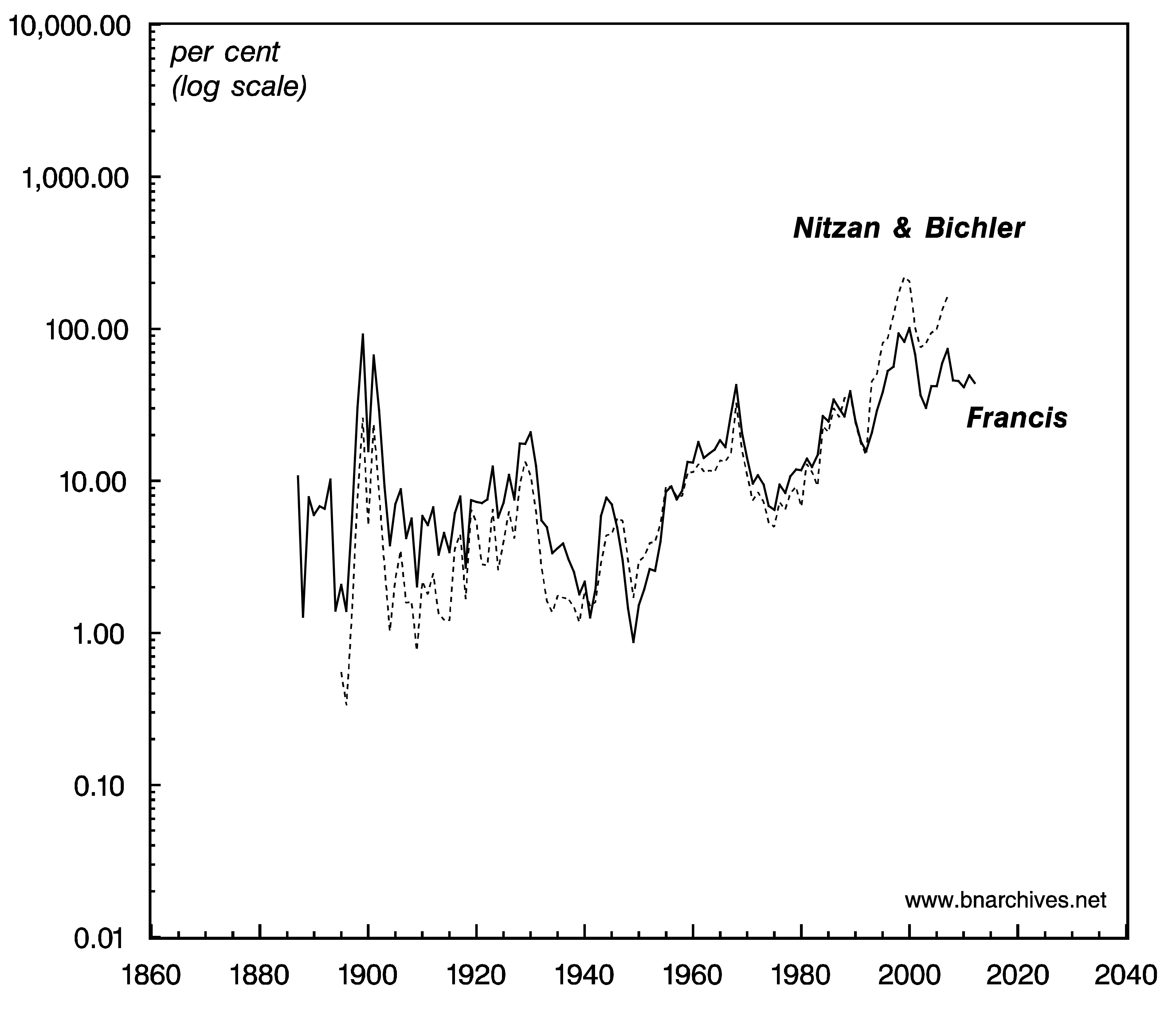
Figure 1: Two Estimates of the U.S. Buy-to-Build Indicator.
NOTE: The last data points are 2012 for Francis’ series and 2007 for Nitzan & Bichler’s series.

SOURCE: Joseph Francis, ‘The Buy-to-Build Indicator: New Estimates for Britain and the United States’; Jonathan Nitzan and Shimshon Bichler, Capital as Power. A Study of Order and Creorder, London & New York, Routledge, 2009.

---

However, in and of itself, the identification of these two sub-periods does not seem to invalidate our original, broader claim; namely, that over the longer haul, the buy-to-build ratio tends to rise.

Both series in Figure 1 show four ‘high points’: (1) the peak of the ‘monopoly wave’ in 1899‑1901; (2) the peak of the ‘oligopoly wave’ in 1929‑30; (3) the peak of the ‘conglomerate wave’ in 1968; and (4) the peak of the ‘global wave’ in 1999-2000. Furthermore, with the exception of the second peak, each ‘high point’ is higher than the previous one — and that relationship holds for both series.

So the key issue is the exceptionally high value of the 1899-1901 peak: does this high value invalidate our claim that the series as whole trends upward?

In our opinion, the answer is no.

The buy-to-build indicator is not like the seemingly eternal business cycle: it has a definite — and fairly recent — starting point. It acquired a positive value probably sometime in the 1870s or early 1880s, when mergers and acquisitions first emerged as a meaningful phenomenon together with the modern corporation and the associated market for corporate equities and bonds. Prior to that point, when there was little to acquire or merge with, the buy-to-build indicator had no clear meaning.

Now, note that Francis’ series begins not in the 1860s or the 1870s, but in the late 1880s, when the value of the buy-to-build ratio was already around 10. Unfortunately, there are no prior data on mergers and acquisitions, so the value of the indicator for earlier years remains known. But we can be pretty certain that during the preceding period the indicator was significantly lower, and that, at some point, it was close to or equal to zero. If we were to prefix Francis’ series with these unknown yet surely smaller numbers, the long-term trend of the full series would have been visibly positive — even with the ‘trendless’ sub-period of 1880-1940.

Figure 2 offers a statistical illustration of these conjectures. The chart plots Francis’ U.S. series for 1887-2012 (solid line), prefixed by an extrapolation of what the earlier data might have looked like (dashed series). To extrapolate the numbers, we make the conservative assumption that the buy-to-build ratio in 1860 was 1 per cent (the actual number was probably lower or even nil). We then compute the exponential growth rate that would have made this ratio reach 10.73 per cent in 1887 (Francis’ first observation). Finally, we multiply the simulated smooth growth series by a random number that is greater than zero but smaller than one, in order to give the extrapolated series the more ragged appearance it probably had.

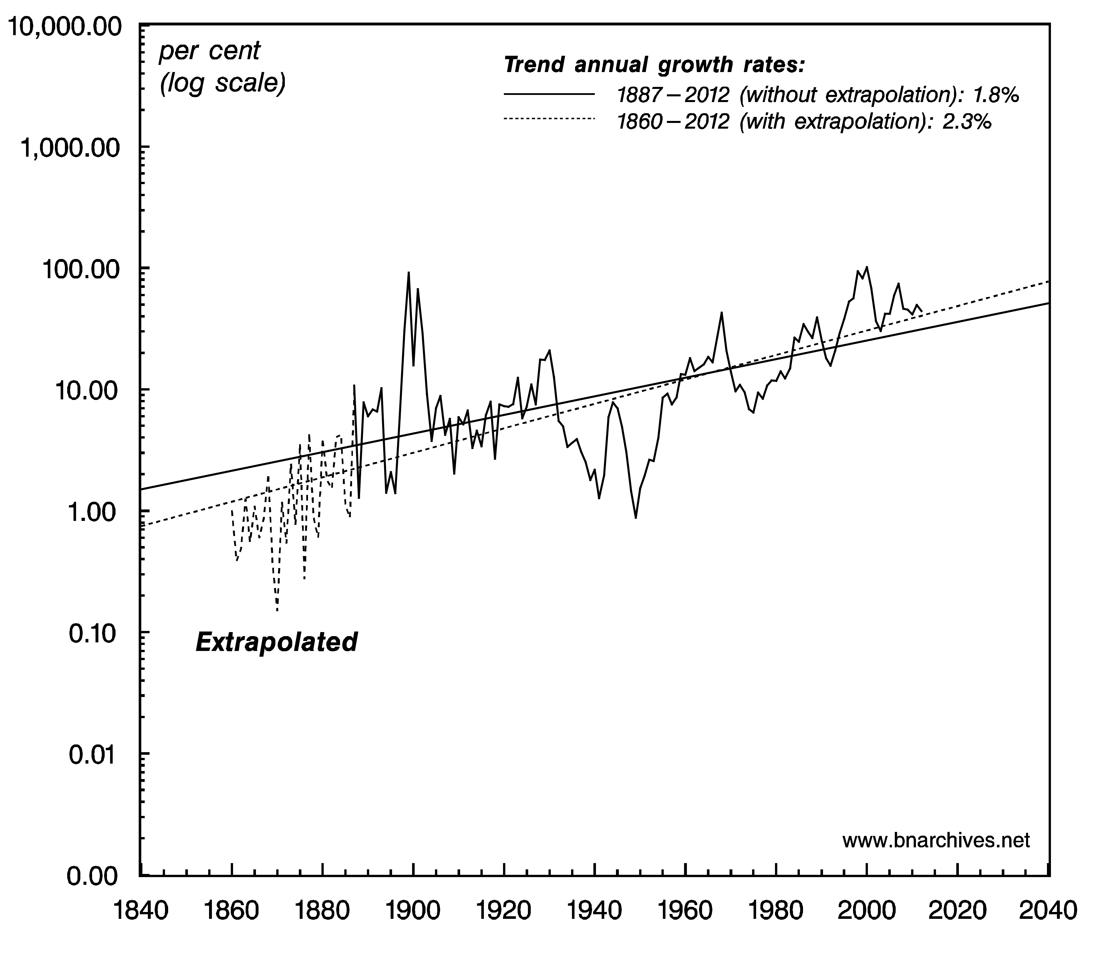
Figure 2: Francis’ U.S. Buy-to-Build Indicator Extrapolated.
NOTE: Data for 1860-1886 are extrapolated in three steps. (1) Set the start value for 1860=1 and the end value for 1887=10.73 (actual value). (2) Impute the 26 missing individual observations for 1861–1886 using a compounded growth factor of 10.73^1/27=1.092. (3) Multiply the imputed observations by a random number 0 < n < 1 to generate a more realistic-looking series. Time trend lines are derived by regressing the log of the series against time and a constant and computing the exponential function of the predicted values. The last data points are for 2012.

SOURCE: Joseph Francis, ‘The Buy-to-Build Indicator: New Estimates for Britain and the United States’; Jonathan Nitzan and Shimshon Bichler, Capital as Power. A Study of Order and Creorder, London & New York, Routledge, 2009.

---

The figure displays two long-term growth trends — one for Francis’ actual estimates (solid line), the other for his estimates augmented by our extrapolation (dashed line). Both trends are positive: the first grows at 1.8 per cent annually, the second at a much steeper rate of 2.3 per cent (setting a smaller value for 1860 would have made the trend growth rate even higher).

Looking at the extrapolated series, it is possible to identify different sub-periods: Francis opines that the period of 1887–1950 is trendless; a second periodization could identify 1860­–1900 as an uptrend and 1900–1950 as a downtrend; a third view could see 1860–1930 as an uptrend and 1930–1950 as a downtrend; and so on. But it seems that, for the period as a whole, and regardless of whether we use the actual or extrapolated series, the long-term trend is positive.

Figure 3 compares Francis’ buy-to-build indicators for the United States and Britain. The long-term trends of the two series are positive and very similar: the annual growth rate of the trend line is 1.8 per cent for the United States and 1.7 per cent for Britain (as for the United States, the growth trend for Britain would have been steeper had we extrapolated the earlier smaller numbers). The two series also move in tandem, with a Pearson correlation coefficient of 0.73 for 1887-2012.

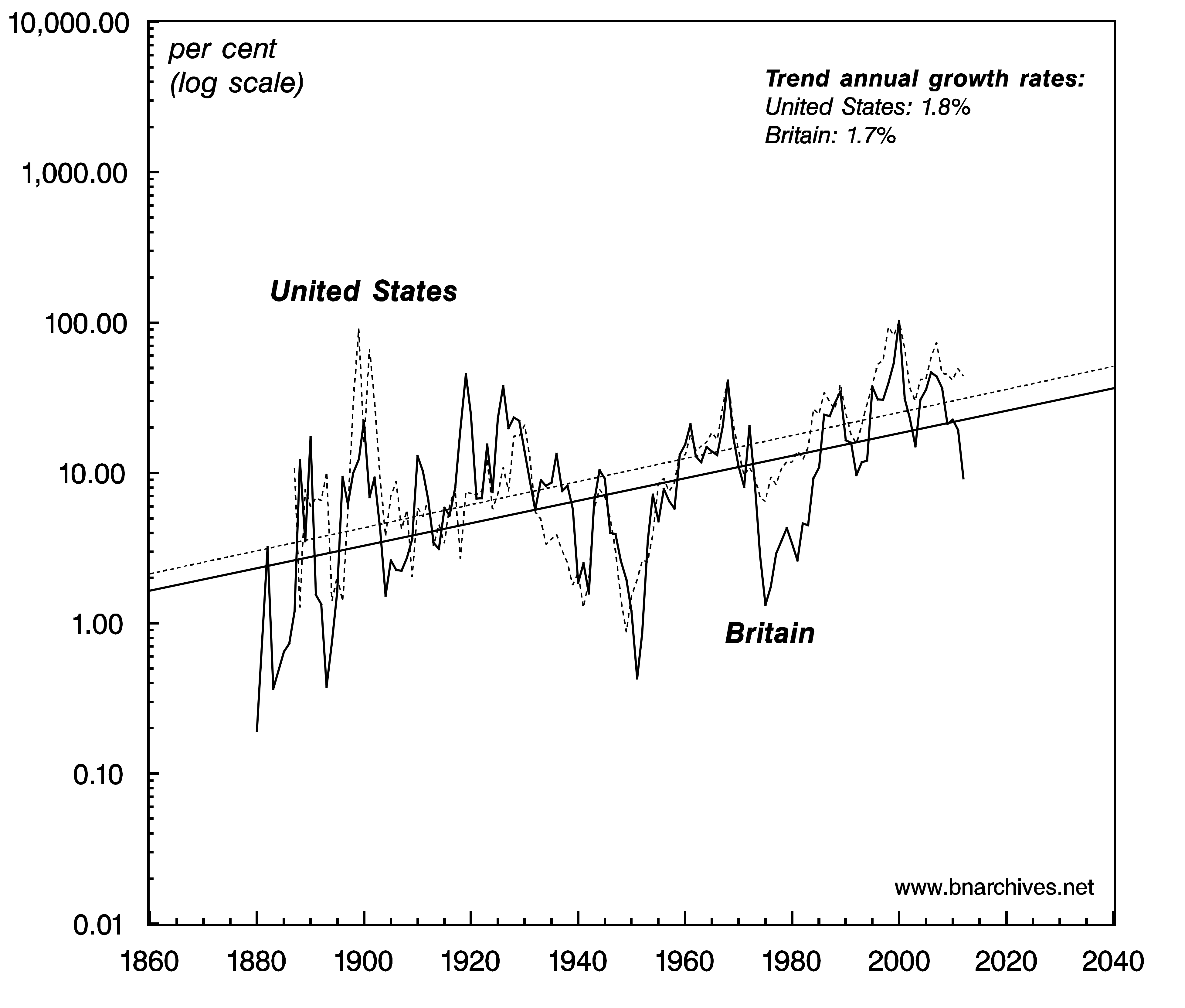
Figure 3: Francis’ Buy-to-Build Estimates.
NOTE: Time trend lines are derived by regressing the log of the series against time and a constant and computing the exponential function of the predicted values. The last data points are for 2012.

SOURCE: Joseph Francis, ‘The Buy-to-Build Indicator: New Estimates for Britain and the United States’.

---

A similar picture emerges from Figure 4, which plots Francis’ stagflation indicators for the two countries. Here, too, there is a tight correlation: 0.69 for 1890-2012. (Note that the stagflation indicator measures deviations from trend, so a value of zero represents the average rate of stagflation for the period.²)

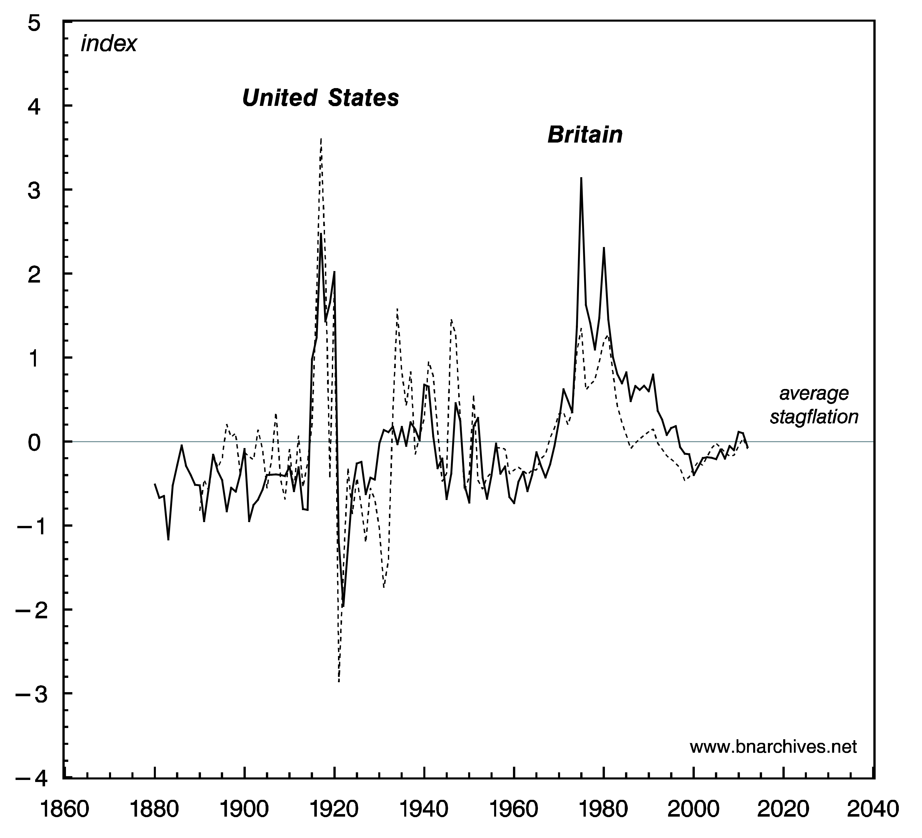
Figure 4: Francis’ Stagflation Estimates.
NOTE: The last data points are for 2012.

SOURCE: Joseph Francis, ‘The Buy-to-Build Indicator: New Estimates for Britain and the United States’.

---

The co-movement and similar trends of the buy-to-build and stagflation indicators in the two countries are significant. They corroborate our suggestion that, over time, the global spread of differential accumulation helps synchronize the breadth-depth cycles across different countries.³ The capital-market integration between the United States and Britain began in the middle of the nineteenth century, and that early start may explain why their breadth-depth cycles already moved in tandem at the turn of the twentieth century.

Notes