Putting Power Back into Growth Theory

Putting Power Back Into Growth Theory

BLAIR FIX

June 2015

Abstract

Neoclassical growth theory assumes that economic growth is an atomistic process in which changes in distribution play no role. Unfortunately, when this assumption is tested against real-world evidence, it is systematically violated. This paper argues that a reality-based growth theory must reject neoclassical principles in favour of a power-centered approach. Building on Nitzan and Bichler’s Capital as Power hypothesis, I argue that hierarchy formation is an integral part of the growth process. I hypothesize that the role of capital accumulation (through profit) is to facilitate hierarchy formation by legitimizing the authority of capitalists.

Keywords

distribution, economic growth theory, energy, hierarchy, power

Citation

Blair Fix (2015), ‘Putting Power Back Into Growth Theory’, Review of Capital as Power, Vol. 1, No. 2, pp. 1-37.

---

Neoclassical growth theory is the dominant approach to understanding economic growth. The canonical neoclassical model — the Solow-Swan model — treats growth as an atomistic process that takes place under conditions of perfect competition. Thus, it assumes that concentrated power plays no role in the growth process. Moreover, neoclassical growth theory assumes that changes in economic distribution have no effect on growth.

This paper has two goals. The first goal is to challenge the validity of neoclassical growth theory by holding its assumptions up to empirical scrutiny. This paper demonstrates that the key assumptions underpinning neoclassical growth theory are systematically contradicted by real-world evidence. The second goal is to offer an alternative approach to growth theory that is consistent with empirical evidence.

This paper provides evidence that a three-way linkage exists between economic distribution, corporate employment concentration, and the growth of energy consumption. If taken seriously, this evidence requires a radical reformulation of the way economic growth is conceived and explained. Rather than being an outcome of atomistic competition, the evidence suggests that growth is fundamentally tied to the accumulation of power. Why? A defining feature of large corporations is their internal hierarchical structure. But since hierarchy (by its very nature) implies a concentration of power at the top, the link between corporate scale and economic scale suggests that growth is inseparable from the accumulation of power.

Like neoclassical theory, this paper hypothesizes that capital accumulation is a key component of the growth process. But while neoclassical theory treats capital accumulation as a physical process, this paper builds on Nitzan and Bichler’s (2009) Capital as Power hypothesis to argue that capital accumulation is an ideological process. Capital is treated not as a ‘factor of production’, but rather, as a social convention that allows the conversion of incommensurable qualities into commensurable quantities. I argue that capital accumulation facilitates hierarchy formation by legitimizing the authority of those at the top. Capitalists exchange capital for institutional ownership — the legitimate right to rule. Thus, capital accumulation perpetuates the authority of owners and allows for the expansion of their power, the formation of larger hierarchies, and increases in energy consumption.

This paper is organized into four sections. Section 1 reviews the key assumptions of neoclassical growth theory, followed by a discussion of the problems associated with using monetary value to measure economic growth. A defining feature of this paper is the use of energy consumption as an indicator of economic scale (rather than conventional ‘real’ GDP). Section 2 presents empirical evidence linking distribution and energy consumption, while Section 3 presents empirical evidence connecting institutional size with energy consumption. Section 4 synthesizes this evidence and presents an alternative vision for economic growth theory.

1     The State of Growth Theory

Neoclassical Growth Theory

Neoclassical growth theory is a logical extension of the neoclassical theory of the firm. The latter treats the firm as a ‘black box’ — all that is known are inputs (labor and capital) and outputs (goods and services). Neoclassical microeconomics posits the existence of a ‘production function’ — essentially a formula — that can explain how the quantities of a firm’s inputs are related to the quantities of its outputs.

Neoclassical macroeconomics applies the same line of thinking to the entire economy: it is the economy that becomes a black box, described only by inputs and outputs. It is posited that a unique aggregate production function exists that can quantitatively explain how capital and labor inputs relate to total economic output. Although there are many varieties of neoclassical growth theory, the Solow-Swan model (Solow, 1956; Swan, 1956) has become the canonical approach (Acemoglu, 2008). At its core is a Cobb-Douglas production function (Eq. 1) in which capital (K), labor (L) and ‘technical progress’ (A) mix together to create material output (Y).¹

Y=AL^{\beta} K^\alpha
(1)

While there are numerous problems with production functions,² for the present discussion, I am concerned with the following two implicit assumptions contained within the Solow-Swan model:

1. distribution is unrelated to growth;
2. large institutions (i.e. concentrated power) are unimportant to economic growth.

I begin with distribution. A central tenet of neoclassical distribution theory is that one’s income is proportional to one’s marginal productivity. When applied to neoclassical growth theory, marginal productivity theory predicts that the exponents \alpha and \beta (in Eq. 1) should be equal to capital and labor’s share of income, respectively. In neoclassical growth theory, it has become standard practice to assume that these exponents are constant.

This tradition has its roots in the work of Cobb and Douglas (1928), who showed that fixed exponents could be used to model historical production. The constancy of ‘factor shares’ was later formalized by Nicholas Kaldor (1957) who put forward a list of six stylized facts about economic growth, one of which was the historical tendency for capital and labor income shares to remain approximately constant over time (about 1/3 and 2/3 respectively). By assuming that returns to labor and capital are constant over time, neoclassical growth theory assumes that changes in distribution do not affect growth.

In order for the neoclassical aggregate production function to be valid, two more assumptions are required: (1) all firms (and the economy as a whole) must experience constant returns to scale; and (2) the economy must be perfectly competitive. Constant returns to scale is a property of a production function Y (K, L) such that increases in the scale of capital and labor inputs yield a corresponding increase in total output. Stated mathematically, this becomes:

Y(cK, cL)= c Y (K, L)
(2)

While, in principle, the production function of individual firms can have either constant, increasing, or decreasing returns to scale, in order to maintain compatibility with the marginal productivity theory of distribution, one must assume constant returns to scale. This assumption arose from an ‘adding up’ problem that neoclassical economists first faced when formulating the marginal productivity theory of distribution. Joan Robinson summarizes this issue: “How do we know that, if each factor is paid its marginal product, the total product is disposed of without residue, positive or negative?” (1934, p. 398).

Using a theorem developed by the mathematician Leonhard Euler, theologian Philip Wicksteed (1894) formulated an elegant solution to the ‘adding up’ problem. He showed that if one assumes that production exhibits constant returns to scale, then Euler’s theorem could be used to ‘prove’ that each factor receives payment in exact accordance with its marginal productivity, thus solving the ‘adding up’ problem.³ As a result of this theorem, neoclassical growth theory (which maintains compatibility with neoclassical distribution theory) is forced to assume that all firms have constant returns to scale. This means that size is assumed to be neither an advantage nor disadvantage: all firms, large or small, are given the same production function.

We now turn our attention to the assumption of perfect competition. Neoclassical theory predicts that under conditions of perfect competition, markets will allocate resources in the most efficient manner possible (given existing patterns of distribution).⁴ Here, perfect competition is used specifically to mean that firms are price-takers: they have no market power that allows them to dictate the price of their output. However, as Coase (1937) noted, this results in a paradox. While the firm is the basic unit of production in neoclassical theory, the theorized efficiency of perfect competition implies that firms should not exist. According to neoclassical logic, the most efficient form of production should occur when competition is most atomistic — when every individual is self-employed.

Given this paradox, why does neoclassical theory continue to assume perfect competition? Steve Keen (2001) argues that it is because without it, the most basic tenet of neoclassical theory — the equilibrium-seeking price mechanism — cannot be justified. Before explaining the problem, let us first review the neoclassical explanation of the market. Arthur Salter says it best:

… the normal economic system works itself. For its current operation it is under no central control, it needs no central survey. Over the whole range of human activity and human need, supply is adjusted to demand, and production to consumption, by a process that is automatic, elastic, and responsive.

(Salter, 1921, p. 15)

In neoclassical theory, the equilibrium-seeking quality of the free market is explained by the forces of supply and demand. Market equilibrium occurs at the intersection of supply and demand curves. These theoretical curves, in turn, are explained in terms of the behavior of individual consumers and producers. The downward sloping demand curve is explained by the law of diminishing marginal utility: a consumer will derive a decreasing amount of pleasure from each additional unit of consumption. The upward sloping supply curve is explained by the law of increasing marginal costs: each additional unit of production is assumed to become costlier to produce.⁵ As long as all firms are price-takers (meaning there is perfect competition), the resulting equilibrium quantity of production is such that the market price equals both the marginal utility of the buyer and the marginal cost of the supplier.

This elegant explanation of the price mechanism underlies all other aspects of neoclassical theory. Yet without perfect competition, it fails to function. If firms have even the slightest market power, then the equilibrium price will diverge from marginal costs, causing the theory to break down. Steve Keen summarizes: “Unless perfect competition rules, there is no supply curve” (2001, p. 101). Thus, the assumption of perfect competition is central to the internal consistency of neoclassical theory. When applied to neoclassical growth theory, this leads to the conclusion that the optimal growth path should be through atomistic competition: large firms should play no preferential role (indeed, they should not exist). This amounts to an implicit assumption that concentrated power plays no role in growth.

To summarize, neoclassical growth theory assumes that distribution and institutional size play no role in economic growth. In the following sections, I demonstrate that these assumptions are directly contradicted by empirical evidence. First, however, I review a major problem (that goes largely unnoticed) facing all economic growth theorists: the accepted measure of economic scale — ‘real’ GDP — is irreconcilably flawed.

Measuring Economic Growth

There is nothing more important to a theory of economic growth than the ability to objectively measure the scale of the economy. Without such a measure, a scientific theory of growth is impossible. Unfortunately, the accepted measure of economic growth — ‘real’ GDP — is plagued by fundamental epistemological difficulties that render it fundamentally subjective.

Any act of measurement begins with an act of reduction. The observer must find a suitable unit for reducing the qualities of the universe to a single quantity. The choice of unit crucially affects this mapping of quantity onto quality. Thus, the concept of economic growth is only meaningful if we can first agree on what it is that is growing. To state formally, measuring material production (Y) can only be done if we reduce it to a single quantity, Q:

Y=Q
(3)

In principle, Q can be defined in terms of any unit. However, before selecting a particular unit, we must present arguments about why this unit is meaningful. Furthermore, for a unit to be effective, it must be socially agreed upon, and it must not change over time and space. Strangely, economists have chosen a unit — price — that does not uphold this simple principle.

The Changing Meter Stick

Let us begin by looking not at the real world of heterogeneous production, but at an imagined world in which production is homogeneous. In this world, only apples are produced, and they are all uniform. In this world, it makes sense to use “apples” as our unit of measurement. If, in the year in question, 300 apples were produced, then:

Y= 300 ~\text{apples}
(4)

Now imagine that our economy begins to produce both 300 apples and 100 oranges (again, all uniform). Now production becomes:

Y= 300 ~\text{apples} + 100 ~\text{oranges}
(5)

This presents a problem: we wish to express Y in terms of a single quantity — but to paraphrase an old adage, you can’t add apples and oranges. We must find a third unit that allows the comparison of ‘apples’ and ‘oranges’. Again, the unit must make sense. For instance, if we were shipping apples and oranges in a truck, a common unit of mass (kg) would make sense. Alternatively, if we simply wanted to eat them, a unit of energy (calories) would be more appropriate.

Since the study of prices is their domain, economists naturally choose monetary value as a common unit of aggregation. This seems reasonable: the price of an orange is much more important to the average person than almost any other metric (mass, energy, etc.).

Keeping with this tradition, we now measure output Y in units of dollars. In order to do so, we must know both the quantity of apples and oranges (Q_A and Q_O, respectively) and their unit prices (P_A and P_O). Production now becomes:

Y= Q_{A}P_{A} + Q_{O}P_{O}
(6)

Using the quantities from above (300 apples and 100 oranges) and adding prices of $3 and $1 for apples and oranges respectively, we get the quantity of production:

\begin{aligned} Y &= (300 ~ \text{apples})( \$3 / \text{apple}) + (100 \ \text{oranges})(\$1 / \text{orange}) \\ &= \$ 900+\$100 \\ &= \$ 1000 \end{aligned}
(7)

Despite the definiteness of our answer, the matter is soon complicated when we realize that our chosen unit (the price of a commodity) changes all the time! For instance, the following year, we might produce the same quantity of apples and oranges, but the price of apples falls drastically to the same price as oranges ($1). Then, without any physical changes, our measure of output is drastically reduced:

\begin{aligned} Y &= (300 ~ \text{apples})(\$1 / \text{apple}) + (100 ~ \text{oranges})(\$1 / \text{orange}) \\ &= \$300+\$100 \\ &=\$ 400 \end{aligned}
(8)

Which one of these measures of material production is ‘correct’? Here lies the fundamental problem: both of them are! By choosing price as an appropriate unit for measurement, we immediately remove the possibility of attaining a single measure for the quantity of output because our unit is not socially agreed upon over time. No amount of intellectual gymnastics can get us out of this dilemma. Without an objective way to decide the year in which prices were ‘correct’⁶ , our measure of economic scale is simply not well defined.

For those who remain unconvinced by this conceptual argument using imagined numbers, we can apply the same reasoning to an empirical example (Fig. 1). Here we use historical quantity and price data for the production of cars and computers (mostly from the United States). Unlike above, now both prices and the physical configuration of production change. Again, we must choose a ‘base’ year in which prices were ‘correct’, and then fix this price across time. This creates a ‘real’ GDP time-series for our 2 product economy. Different choices of base year drastically change the way we conceive of output growth.⁷ Indeed, the economy simultaneously grows considerably and hardly at all!

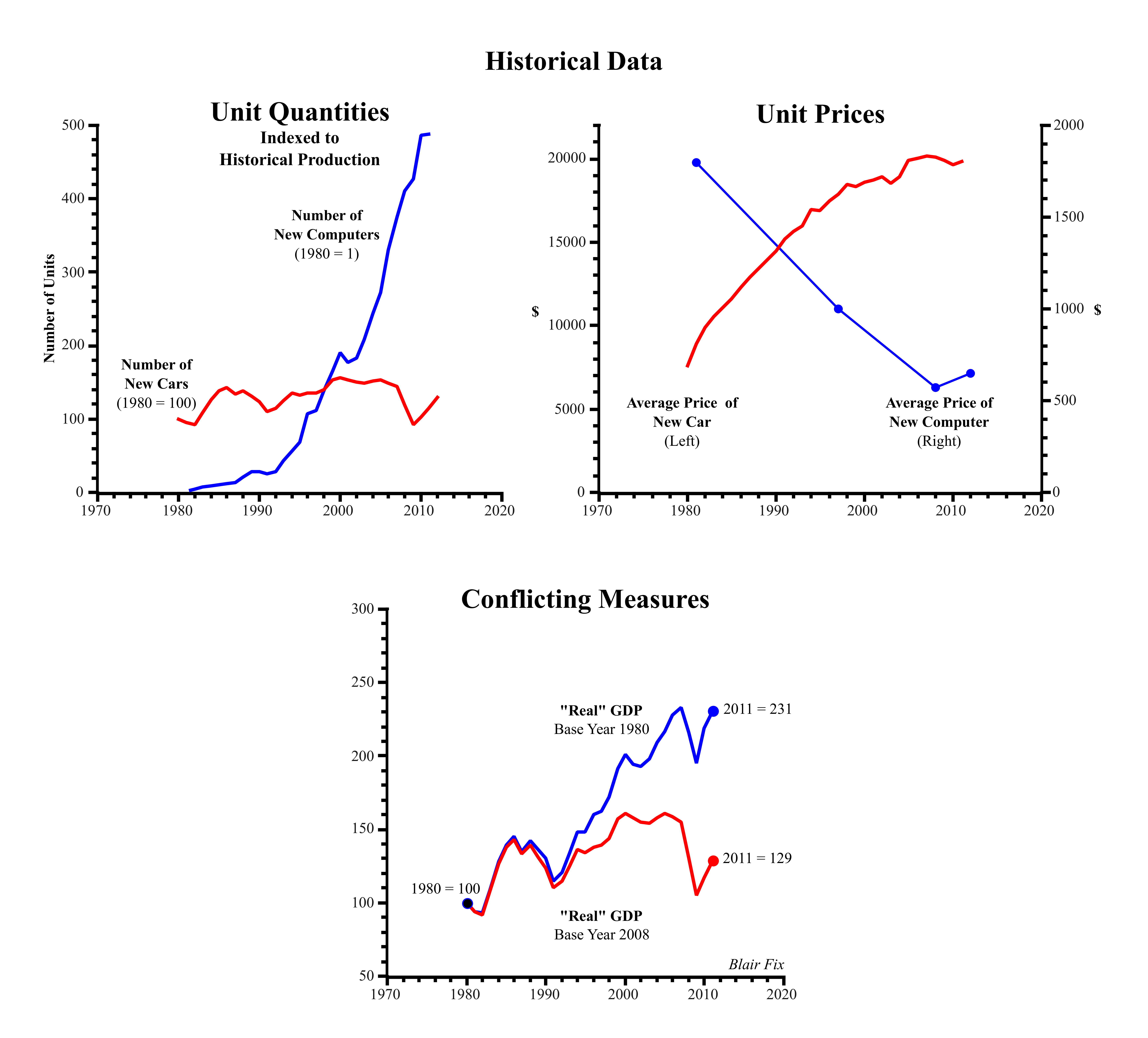Figure 1: Measuring Production with a Changing Meter Stick.
Note: This methodology is modeled after critiques of capital aggregation offered by Nitzan & Bichler (2009). Sources: Quantity of cars from Ward’s Automotive Group, “U.S. Car and Truck Sales, 1931-2012” at wardsauto.com/public-data. Quantity of computers from Jeremy Reimer, Total Share: Personal Computer Market Share 1975-2010, jeremyreimer.com. Price of cars from Bureau of Economic Analysis, Table 10.11, Average Price of a New Car, 1970-2011 (using domestic prices). Computer prices are from the Wikipedia entry for personal computer. Note: computer price indices from US Bureau of Labor statistics are unsuitable here because they adjust for changing computer quality (ie: processor speed, memory, etc.).

---

A further difficulty with real GDP methodology is that commodities change qualitatively over time. Neither the computers nor the cars of 1980 looked anything like those of 2010. In order to combat this problem, statistical agencies attempt to measure these qualitative changes. However, we again encounter a number of fundamental problems. Firstly, we must subdivide a given commodity into relevant attributes. But how do we objectively decide those attributes that are relevant and those that are irrelevant?

Furthermore, once we have reduced a commodity to its constituent attributes, how do we decide their relative importance? The most popular method is called hedonic quality adjustment. The Bureau of Labor Statistics summarizes the process as follows:

In price index methodology, hedonic quality adjustment has come to mean the practice of decomposing an item into its constituent characteristics, obtaining estimates of the value of the utility derived from each characteristic, and using those value estimates to adjust prices when the quality of a good changes.

(Bureau of Labor Statistics, 2010, emphasis added)

All quantitative comparisons require a unit of measurement. Here we see that the Bureau of Labor Statistics is attempting to measure the attributes of a commodity in units of utility. This is problematic because utility (a hypothetical psychic flux) cannot be directly measured; rather, it must always be ‘revealed’ through prices (Samuelson, 1938). Thus, hedonic measurement becomes circular: distinguishing changes in price from changes in quality requires knowledge of consumer preferences; however, consumer preferences can be measured only through prices.⁸

To summarize, when measuring the quantity of production in terms of prices, we fall victim to a changing meter stick. When measuring changes in the quality of a commodity, our unit cannot actually be measured independently of prices. The logical choice at this point is to abandon prices as a unit for quantifying material output. A more appropriate approach — one that meshes nicely with the current state of scientific knowledge — is to use energy as our unit.

Energy and the Thermodynamic Basis of Growth

Using energy as a metric for growth is logical for two reasons: firstly, the units are well defined; and secondly (and most importantly) it is physically meaningful. Astrophysicist Eric Chaisson (2002) writes that “[e]nergy — the ability to do work, or to cause change — is the most universal currency known in natural science”. What seemed like separate phenomena 200 years ago — heat, motion, light, electricity, magnetism, chemical potential — are now recognized to be different forms of a universal property we call energy. The science of energetics has made great advances in understanding and quantifying energy in its many forms. Because of its universality, energy is especially useful for the study of seemingly disparate processes.

There is virtually unanimous agreement that energy flows form the basis for all biological life (Kondepudi & Prigogine, 1998; Lotka, 1956; Morowitz & Smith, 2007; Odum, 1988; Schrodinger, 1992). Life is a subset of what are referred to by physicists as ‘non-equilibrium structures’. Equilibrium, in thermodynamics, is the state towards which all isolated systems evolve. This state of maximum entropy can be thought of as the most boring situation imaginable — homogeneous temperature and pressure, no changes over time, and no organized structure.

Without flows of energy, all roads lead to equilibrium. However, the flow of energy through a system leads to the permanent departure from equilibrium and can cause the emergence of complex ‘dissipative structures’ (Kondepudi & Prigogine, 1998). Along with single organisms, the notion of a dissipative structure can be extended to include ecosystems and human societies. Indeed, the importance of energy to human societies is well-recognized (Cottrell, 2009; Debeir, 1991; Georgescu-Roegen, 1971; Hall & Klitgaard, 2012; Smil, 1994). The laws of thermodynamics indicate that for a human society to increase its biophysical scale, it must consume more energy. It only makes sense, then, to use energy as a metric for growth.

Measuring energy consumption, however, is not without difficulties: we must decide ‘where’ to measure energy flow. I use the word ‘where’ not in the spacial sense, but in the conceptual sense. The use of energy involves numerous transformations into numerous forms. Pre-analytic decisions about accounting methodology will drastically change our final results.

This can be illustrated by following the energy required to power a car (Fig. 2). In our example, fossil fuel energy initially enters the economy in the form of crude oil. The crude oil is then transformed into gasoline, which involves some energy losses. The gasoline is burned in an internal combustion engine (turning chemical energy into thermal energy) before ultimately being transformed into the kinetic energy of an automobile. At each stage of this process, energy is lost. Thus, depending on ‘where’ we measure its flow, we’ll get very different data for the consumption of energy.

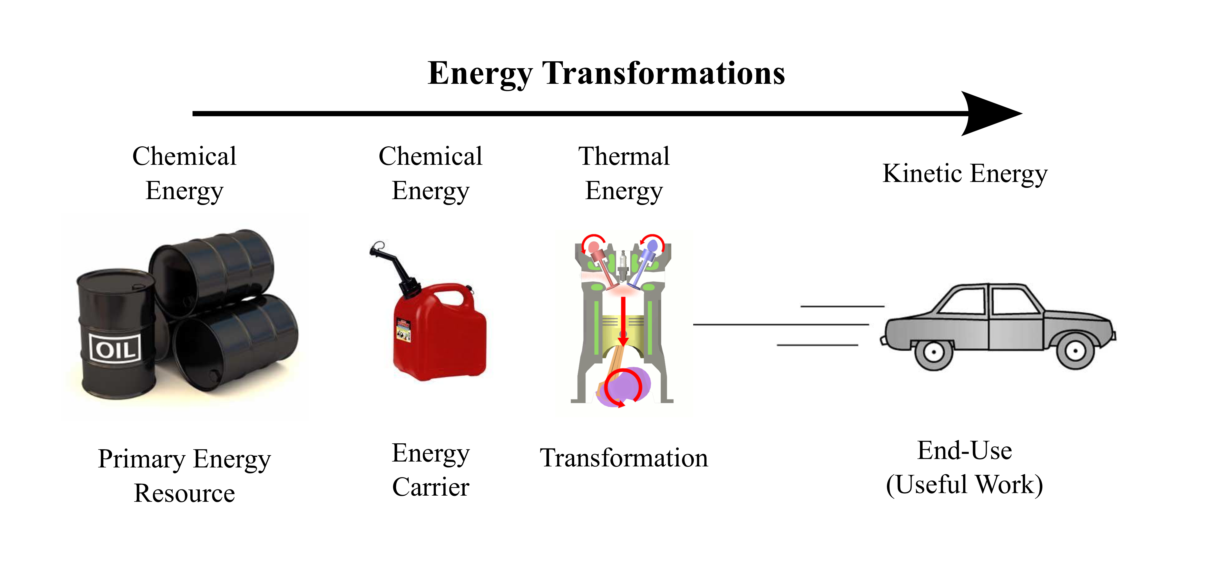Figure 2: ‘Where’ to Measure Energy Consumption?

The most straightforward ‘place’ to measure energy consumption is as it enters the economy as a primary energy resource (most statistical agencies use this method). Since there are relatively few varieties of primary energy, this type of accounting is relatively easy.⁹ As we move towards end-use energy, accounting becomes increasingly complex, as the number of potential categories grows astronomically.

While some scholars argue that quantifying end-use energy is impossible (Giampietro, Mayumi, & Sorman, 2013), Robert Ayres and Benjamin Warr (2005) have made a laudable first attempt, calling their result ‘useful work’. While I will not discuss the details of their methodology here, the process involves a conceptual simplification of the types of end-use categories and a calculation of the aggregate efficiency of each category (in a given year).¹⁰

The purpose of Ayres & Warr’s useful work calculation is to enter it into a production function capable of hind-casting the growth of ‘real’ GDP (Ayres & Warr, 2010). Indeed, numerous scholars have made the link between growth in energy consumption and the growth in GDP (Cleveland, Costanza, Hall, & Kaufmann, 1984; Cleveland, Kaufmann, & Stern, 2000; Garrett, 2012; Hirsch, 2008; Stern, 2011). All studies show a high correlation between the two. Few scholars, however, have made the conceptual leap that I make here: that energy is a valid growth metric unto itself.

I assert that useful work stands on its own as one of the best metrics of biophysical scale. For the rest of the paper I use energy consumption as my metric for the biophysical scale of the economy. When data is available, I use Ayres & Warr’s useful work metric. When such data is unavailable, I simple use primary energy consumption.

2     Distribution and Growth

My goal is to connect changes in useful work to changes in economic distribution. However, any discussion of distribution must begin by defining the types of income. Modern systems of national accounts allocate income into five main categories: wages, proprietor, rent, interest, and profit. Each type of income is accompanied by a particular institutional arrangement, explained below.

The Types of Income

Wages

Wages accrue to workers who ‘own’ their labor power but who do not own what they produce (Marx, 1867). Since ownership is defined as an act of enclosure, this implies that a wage earner must have the ability to restrict access to his/her labor. Workers who do not earn income have either lost this ability (i.e. slaves) or have decided not to enforce it (i.e. domestic labor or volunteer work). The enclosure of human labor can be magnified through group coordination in the form of unions and combinations. By refusing to work, these groups of workers reinforce the enclosure of their labor, thereby strengthening their bargaining position.¹¹

Proprietor

Sole-proprietors¹² own their labor and the things they produce. The classic example of the sole-proprietor was in the so-called ‘putting-out’ system of early capitalism (Polanyi, 1964). Rural inhabitants produced goods that they then sold. Thus, the clearest distinction between sole-proprietorship and wage labor can be made by contrasting the putting-out system with the factory system: in the latter, workers clearly do not own what they produced, while in the former they do.

Rent

Rent implies ownership of a specific ‘thing’. Thus, rent accrues to owners of land, infrastructure, and natural resources. However, it can also be earned by owning less tangible things like intellectual property. In the US national accounting system, rent can only flow to a person, not an institution. Thus, when corporations or sole-proprietorships earn income by renting out property, it is automatically called profit or proprietor income (respectively).¹³

Profit

Profit flows to the owners of business equity. This is a more abstract form of income than rent, as it implies ownership of a legal structure rather than a specific piece of property. In return for owning this equity, owners gain a say in business decision-making.

Interest

Interest flows to those who own debt. By lending money, a creditor essentially purchases the rights to a future income stream — interest. In this sense, interest is associated with the most abstract form of ownership — ownership of nothing but an income stream itself. Modern business practices have made the distinction between profit and interest (equity and debt) difficult to discern. However, there are important differences. Firstly, debt offers a fairly stable rate of return (dictated by interest rates), while profit is often volatile. Secondly, owners of debt (unlike owners of equity) have no decision-making authority unless the company enters receivership.

The Differential Growth of Income

Now that we have defined the various types of income and attributed them to specific types of ownership, we can move on to the task of connecting them with growth. I ask the following question: under a growth regime, who are the relative winners and who are the relative losers? In order to investigate this question, I follow Nitzan & Bichler (2009) in discarding the use of ‘real’ metrics of income in favor of differential ones. I conceptualize different types of income as slices of a giant pecuniary pie (Fig. 3), and then investigate relative changes in the size of each slice. The goal is to compare these changes to the rate of economic growth.

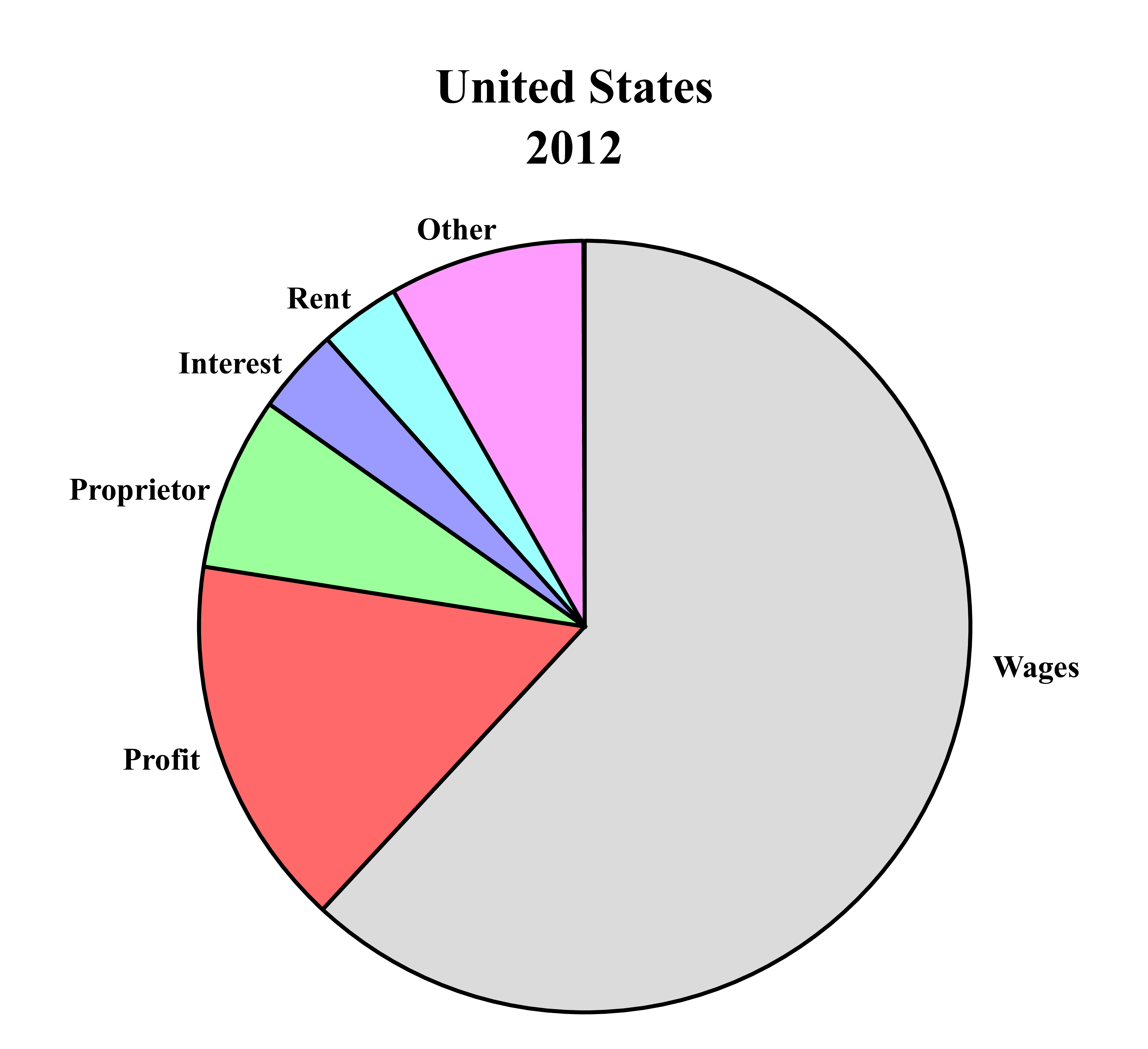Figure 3: The Pecuniary Pie.
Source: Bureau of Economic Analysis, Table 1.12, National Income by Type of Income.

---

I begin by explicitly stating my methodology. Equation 9 shows a sample calculation for wages. On the left side, we divide useful work (U) by population (P) to get useful work per capita. We then calculate the annual growth rate — signified by the hat symbol ( \widehat{ ~ } ). We then compare this to the rate of change of the wage bill (W) as a portion of national income (NI) (right side).

\widehat{\left[\frac{U}{P} \right]} \Longleftrightarrow \widehat{\left[\frac{W}{NI} \right]}
(9)

The results for this methodology, carried out over the 5 classes of income, are displayed in Table 1 in descending order of correlation. Positive correlation indicates that positive growth rates of useful work are associated with differential increases in the income-type in question. Conversely, negative correlation ( - ) indicates that positive useful work growth rates are associated with a differential decrease in that income-type.

Table 1: Correlation Between Income Redistribution & Growth

Income Type	\boldsymbol{R^2}
Profit	0.52
Interest	(–) 0.28
Rent	(–) 0.16
Wages	(–) 0.15
Proprietor	0.08

The results are striking: the growth of useful work overwhelmingly occurs under conditions in which income is redistributed towards profit (Fig. 4). But what is so special about profit? Why is it the only income-type for which differential changes are positively correlated with growth? To answer this question, we must investigate the institutional context under which profit-making occurs.

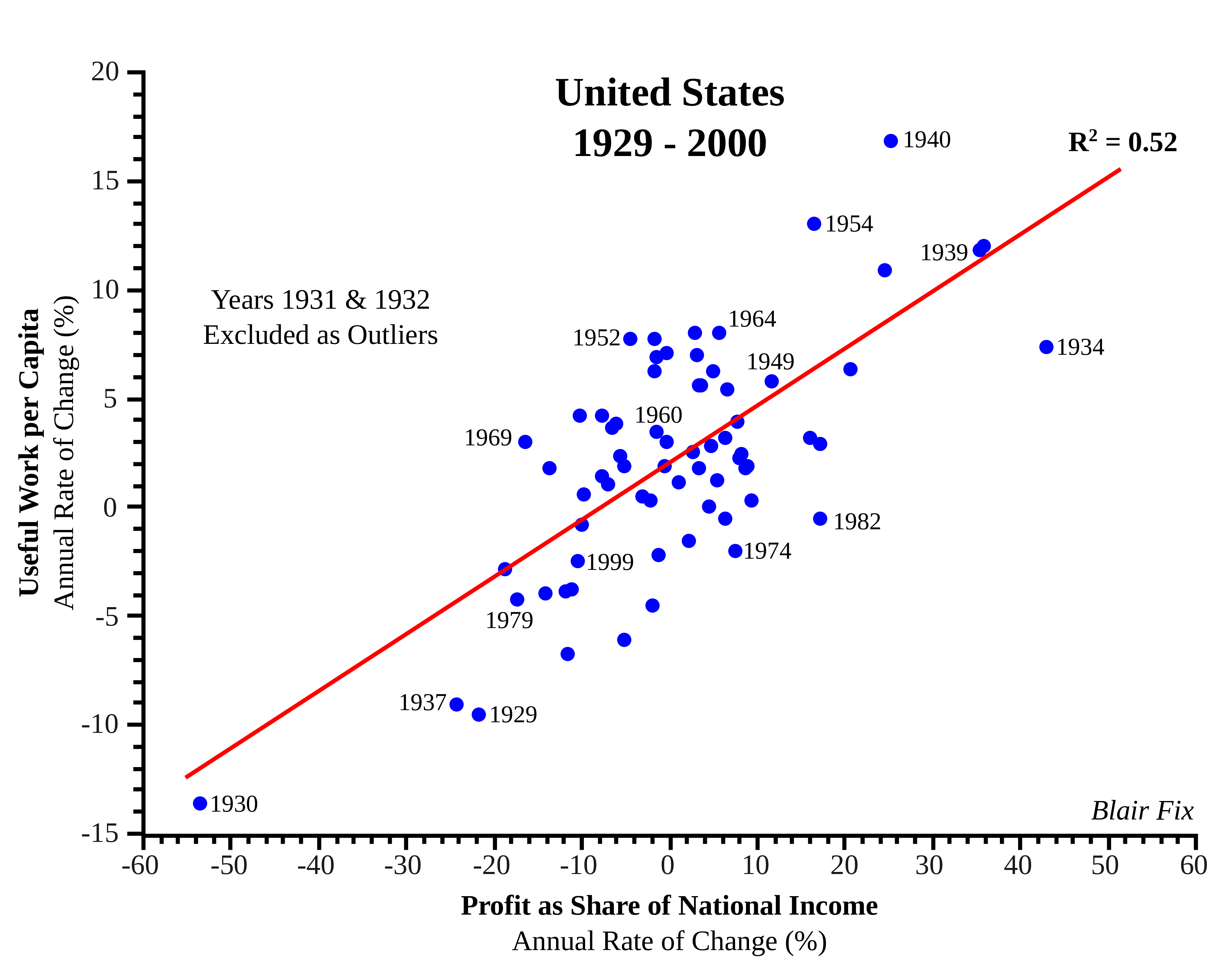Figure 4: The Growth of Useful Work vs. Redistribution Towards Profit.
Sources: Data for useful work is from Benjamin Warr’s REXS database (and is available only for the period 1900-2000). Profit and national income data are from BEA Table 1.12, National Income by Type of Income.

---

3     The Institutional Context

I begin with a simple truism: if a change in economic distribution is to have any effect on a society, it is because this change moves money (and power) into different hands. Of course, this seems trivial — what is a change in distribution if not a change in who controls what? However, I argue that it is only when profit is coupled with hierarchy that a relative change in profit moves money and power into different hands. In all other institutional arrangements, introducing/increasing profit has no discernible effect on who controls what — it merely shifts the way that money is accounted on paper.

Before I proceed, let me first discuss how to interpret Figures 5–7. Each figure contains a visualization of a specific form of institution. On the left-hand side, the black arrows show an income stream that flows to the institution. This income is then split into different accounting categories that vary according to the type of business. All businesses incur non-labor costs, which flow to other individuals or institutions (where they count as income). The rest of the income stream is divided between profit, salary/wages, or proprietor’s income. Wages and proprietor’s income flow directly to individuals, while profit flows to the owners of institutions (dotted lines). The dotted red line represents decision-making power over how the original income stream is split. In each example, the arrows are labelled by accompanying percentages, signifying the hypothetical size of the flow in relation to the original income stream.

The Types of Institutions:

Atomistic Institutions

Atomistic institutions consist of a single, self-employed person (Fig. 5). There are two possible configurations: the sole-proprietorship or the self-employed individual who incorporates his/her business. Modern accounting principles dictate that a sole-proprietor’s income be called ‘proprietor income’, and not profit. However, the distinction is in name only — both profit and proprietor income are defined as the total sales less the costs of doing business. If a self-employed individual incorporates, this allows for a conceptual (and legal) separation of income into ‘profit’ and ‘salary’.

Figure 5: Atomistic Institutions.

There are two main benefits to incorporating. Firstly, corporations are limited liability institutions, which allows a legal separation of business and personal assets. In the event of a bankruptcy, only business assets can be seized. The second benefit is that profit is generally taxed at a different rate than a salary. For instance, in 2011, the effective US corporate tax rate was 21%, while the highest tax rate for personal income was 35%.¹⁴ Despite these differences, the two forms of business displayed in Figure 5 are, for all intents and purposes, the same.

Let us envision a society populated only by these two institutional configurations (similar to the one imagined by Adam Smith (1776)). We ask the following question: what is the effect of redistributing income from wages and proprietor income towards profit?

There are two possible ways for this to occur. The first is if a sole-proprietor decides to incorporate his/her business. This would eliminate his/her proprietor income from the national accounts, but add wage and profit income in the same amount. The effect would be a change on paper, but no meaningful change in who actually controls this income (the same person in both cases). Alternately, a self-employed person with an incorporated business might decide to allocate more income to profit rather than to salary (if tax rates changed, for instance). Again this has no meaningful effect outside of a re-categorization on paper: in both cases the individual’s total income remains unchanged.

For a society populated entirely by atomistic institutions, it is difficult to see how an income redistribution towards profit would change anything but the abstract accounting category used to classify income.

Flat Institutions

We now move on to institutions that include more than one person. We begin with non-hierarchical, or so-called ‘flat’, institutions (Fig. 6). A flat institution is characterized by a complete lack of hierarchy. In its ideal form, this means that each individual has an equal say in all decision-making processes. Our hypothetical, flat institution can either be operated as a non-profit organization (i.e. a cooperative), or as a flat corporation (with ownership divided equally among its members). In the former case, all income in excess of costs is allocated to salaries, while in the latter case, this income is split between profit and salaries.

Figure 6: Flat Institutions.

As we did previously, we imagine a society populated only by such flat institutions. Again, we ask: what is the effect of a redistribution of income towards profit? This could occur two ways — either by non-profits deciding to become for-profit, or by for-profits increasing their markup (profit as a portion of total income). In neither case does this change affect the ultimate control of the pre-existing income stream (which is always allocated equally to all individuals). However, the re-categorization of salaries into profit does have the effect of pooling income. For instance, having a group of 5 people control $100 000 in profit is different than having each of those 5 people control $20 000 in salaries. Pooling income allows for the possibility of a larger ‘investment’ than would be possible otherwise.

However, the ability to pool income does not require profit. Indeed, the initial income stream is the ultimate source of any pooled income. Thus, if a co-operative wishes to make a large purchase, it may simply divert more of its income stream towards ‘costs’ and less towards salaries. The end result is the same.

As we did with single-person institutions, we reach the conclusion that when profit only flows to flat institutions, an income redistribution towards profit should have no effect outside of a change on paper.

Hierarchical Institutions

We now move on to hierarchical institutions (Fig. 7). Here we envision the quintessential hierarchy that is marked by a strict top to bottom chain of command, with all decision-making power ultimately residing at the top. We have two possible types of institution — the hierarchical non-profit and the hierarchical corporation. A good example of hierarchical non-profits are state-owned companies like Fannie Mae or PetroChina, while Walmart and General Motors are examples of hierarchical corporations.

Figure 7: Hierarchical Institutions.

As before, we are interested in the effect of redistributing income towards profit, but now in a society populated entirely by hierarchical institutions. There are two possible scenarios: either a non-profit organization may become a for-profit (as when a state-owned company is privatized) or a for-profit organization could increase its markup. Unlike our previous examples, here both scenarios imply a significant change in who controls what. A differential increase in profit will serve to concentrate income at the top of the chain of command.

The results of our conceptual investigation demonstrate that it is only when coupled with hierarchy that a redistribution towards profit has any meaningful effect on who controls what. In all other institutional settings, introducing/increasing profit has no effect beyond a shift in abstract accounting categories.

Connecting Hierarchy, Distribution, and Growth

Given the empirical link between redistribution and the growth of energy consumption, and our finding that relative changes in profit are only meaningful if they occur within a hierarchical institution, it seems logical to look for connections between hierarchy, profit, and growth. To do so, we must decide on a metric for hierarchy. Inspired by Nitzan and Bichler’s (2009) concept of ‘breadth’, I propose using the employment share of the largest n corporations as such a measure (where n is an arbitrary number chosen based on data availability). The logic underpinning this metric is straightforward: large corporations are hierarchical institutions; therefore, the extent to which such corporations dominate total employment should give us an indication of the ‘degree of hierarchy’ of society (keeping in mind that this hierarchy is always internal to corporations).

Hierarchy and Growth

In order to connect hierarchy and growth, I continue to use energy per capita as my metric for growth. However, due to the lack of data at the global level, I use primary energy consumption, rather than useful work. My methodology is straightforward: I simply compare corporate employment concentration to energy use per capita and look for correlation. The results of this analysis, undertaken first at the international level (Fig. 8) and then at the national level (Fig. 9), demonstrate a clear connection (across both space and time) between corporate employment concentration and energy consumption per capita.

Figure 8: Global Corporate Employment Concentration vs. Energy Use.
Sources: National energy use per capita and total labor force data is from the World Bank (indicator codes EG.USE.PCAP.KG.OE. and SL.TLF.TOTL.IN, respectively). Employment of top 10 corporations (ranked by number of employees) is from COMPUSTAT Global Fundamentals (series EMP).

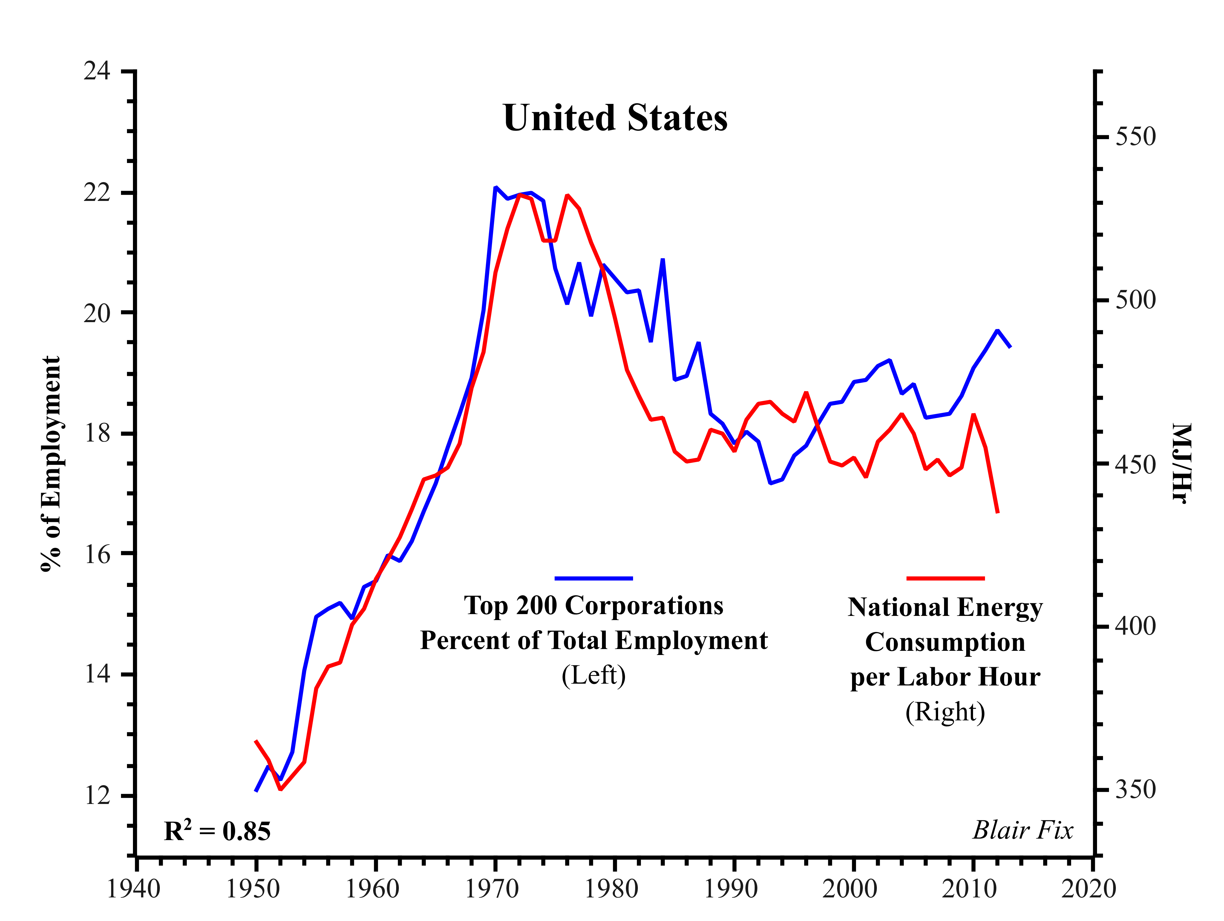Figure 9: US Corporate Employment Concentration and Energy Use per Capita.
Sources: Total US employment from BEA Tables 6.5 B-D (Full-Time Equivalent Employees by Industry). Employment of top 200 corporations (ranked by number of employees) from COMPUSTAT (series DATA29). Total energy consumption from EIA Table 1.3 (Primary Energy Consumption by Source). Total labor hours from BEA Tables 6.9 B-D (Hours Worked by Full-Time and Part-Time Employees by Industry).

---

From a neoclassical perspective, this finding is puzzling. Indeed, neoclassical growth theory assumes that concentrated power should play no role in the growth process. The evidence, however, suggests just the opposite: growth is consistently associated with an increase in the control of large corporations. That is to say, growth and the concentration of power appear to be intrinsically related.

Hierarchy and Profit

So far, I have empirically connected relative changes in profit to changes in energy consumption, and I have empirically connected changes in hierarchy to changes in energy consumption. The last piece of the puzzle needed to create a three-way connection between hierarchy, profit and growth, is to link relative changes in profit to changes in hierarchy. In order to do this, I turn to capitalist income, which consists of the sum of profit and interest. An important question to ask is — does the composition of capitalist income (the balance between interest and profit) affect hierarchy formation?

Political economists have long sought to understand the differences between interest and profit. In Marxist political economy, interest is generally regarded as parasitic,¹⁵ and profit (while exploitative) is regarded as productive. However, Nitzan and Bichler (2009) challenge this long-held belief by arguing that neither profit nor interest is productive. According to Nitzan and Bichler, a return on capital is the result of an owner’s strategic ability to control (restrict) human activity (through a property rights regime). Interest and profit simply represent different ways of earning a return on capital. Nitzan and Bichler argue that interest represents the ‘normal’ rate of return, while profit offers the chance to beat this normal rate.

While debt holders (who earn interest) and equity holders (who earn profit) should both be considered ‘owners’ of a corporation, there is an important legal difference between the two forms of ownership. Other than when a corporation is in receivership, debt holders have no legal control over business decisions — it is equity holders that have this right. If a particular equity holder owns enough stock (and often owning only a small fraction of outstanding stock is enough) he or she has complete control of business decision-making. If we think of this in terms of hierarchy, then it is clear that equity holders (with controlling shares) are at the top of the corporate pyramid. Debt holders, on the other hand, are only at the top if a corporation files for bankruptcy (i.e. during periods of crisis).

It seems reasonable to hypothesize that the balance between profit and interest might have some effect on the behavior of capitalists. Since profit is associated with ‘active’ ownership, perhaps the balance between profit and interest will be reflected by changes in the rate at which corporate employment concentration changes. Figure 10 examines this hypothesis by plotting the annual rate of change of US corporate employment concentration (smoothed with a 10 year moving average) against the share of profit in capitalist income (the sum of profit and interest, also smoothed with a 10 year moving average).

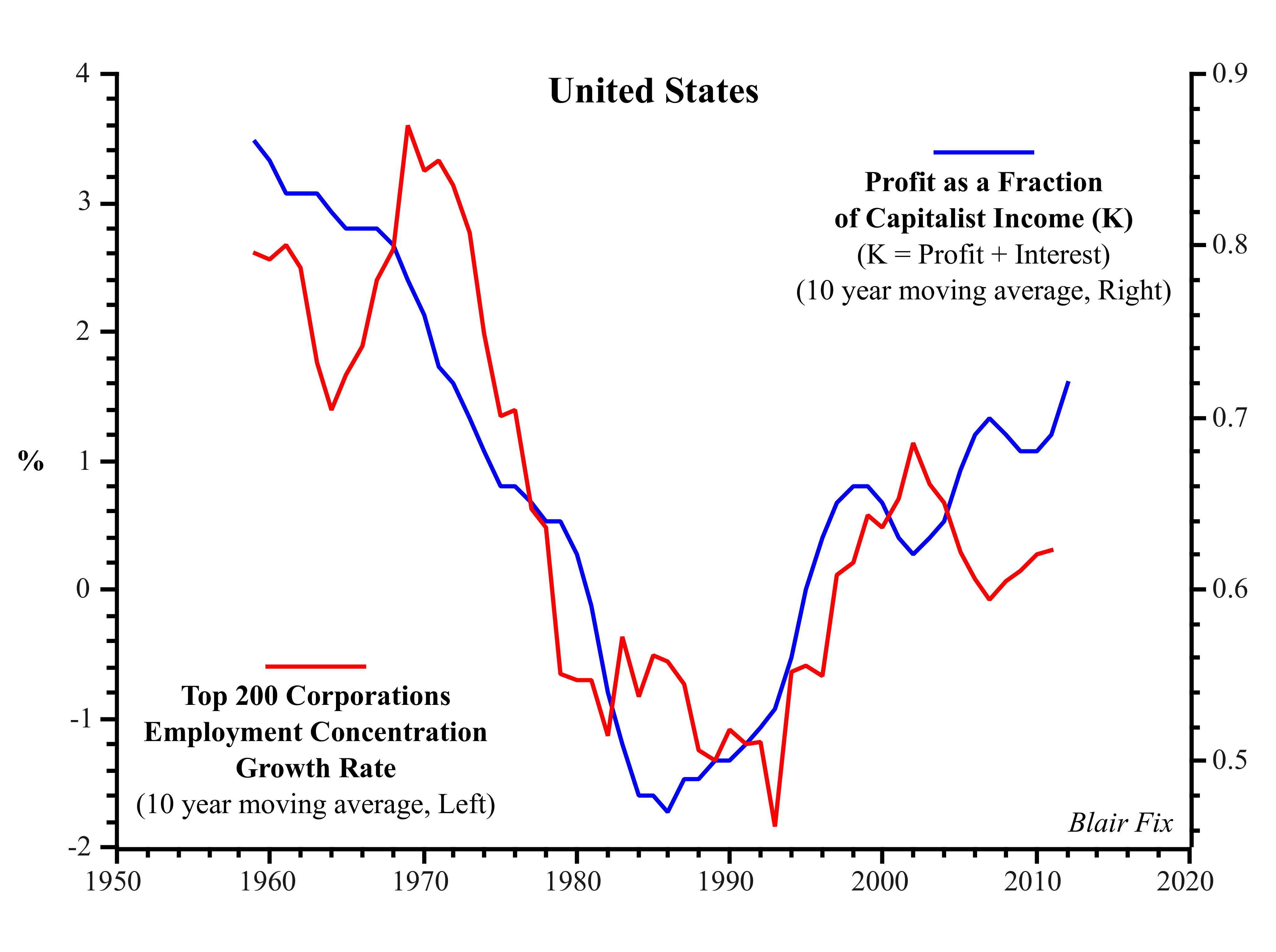Figure 10: Connecting Profit to Corporate Concentration.
Sources: Total US employment from BEA Tables 6.5 B-D (Full-Time Equivalent Employees by Industry). Employment of top 200 corporations (ranked by number of employees) from COMPUSTAT (series DATA29). Profit and Interest from Bureau of Economic Analysis, Table 1.12, data series: Corporate profits with IVA and CCAdj, Net interest and miscellaneous payments.

---

The correlation is clear: corporate concentration (i.e. hierarchy) grows more rapidly when capitalist income is dominated by profit, and more slowly when capitalist income is dominated by interest (R² is 0.70 for smoothed data, 0.17 for raw data). Profit, it would seem, is key for hierarchy formation.

4     Putting Power Back into Growth Theory

Having established a three-way link between profit, hierarchy and growth, I now offer my own hypotheses about why this connection exists. While speculative at this point, these hypotheses offer plausible grounds for future inquiry.

Hierarchy and Group Size

The evidence suggests that the growth of energy consumption requires the formation of large, hierarchical organizations that are capable of mobilizing vast groups of people towards a unified objective.¹⁶ But why is this the case? Why can’t growth be accomplished by the random interactions of atomistic institutions (as neoclassical theory suggests)? One possible explanation (which I pursue here) is that humans have evolved to function in small, egalitarian groups. Without coercive, centralized power, such small-scale groups will not be able (or willing) to coordinate their actions. In order to coordinate larger groups of people, egalitarian relationships must be abandoned in favor of hierarchical ones. Recent anthropological research supports the hypothesis that egalitarian group size is fundamentally constrained by human brain size.

The ability to form social groups is, in large part, a function of genetic inheritance. This becomes obvious when we compare different species: many animals (such as bears) are incapable of forming large groups, while others (such as wolves) do so naturally. All social organisms have evolved mechanisms that maintain the cohesiveness of their groups. In primates, it appears that this has involved the development of large brains.

In a remarkable study, anthropologist Robin Dunbar (1992) found that the group size of different primates was highly correlated with the relative size of their neocortex (Fig. 11). His conclusion was that neocortex size places an upper limit on the number of social relations that can be monitored by an individual. That is, since managing social relationships requires computational ability, brain size imposes a limit on group size. From his results on non-human primates, Dunbar (1993) extrapolates to find that human brain size predicts a group-size limit of about 150 (often called ‘Dunbar’s number’). While this number should be considered exploratory, Dunbar notes that Neolithic villages had populations in this order of magnitude. Clearly, however, humans have developed ways of vastly exceeding this social scale: modern cities can surpass Dunbar’s number by five orders of magnitude.

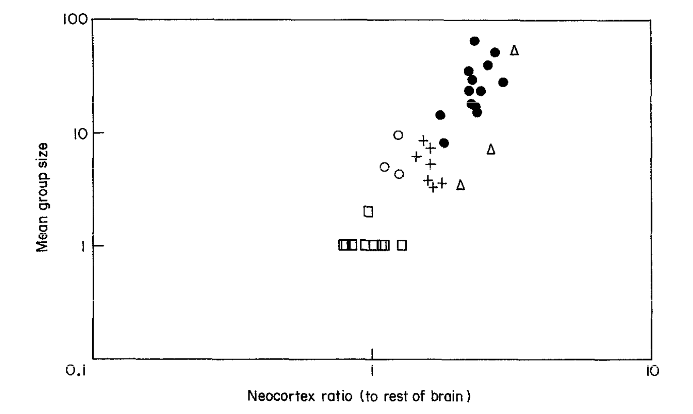Figure 11: Primate average group size vs. neocortex size.
Note: Plot icons (squares, circles, etc.) represent different primate genera. Neocortex size is measured in terms of its volume relative to the rest of the brain. The neocortex is the largest and evolutionarily most recent portion of the brain and is the site of most of the higher brain functions. Source: Dunbar (1992).

---

If we accept Dunbar’s hypothesis, it follows that any mechanism that allows vast increases in group size must function to limit internal interactions between group members. Neoclassical theory attempts to prove that ‘the market’ is the ultimate organizational mechanism. Unfortunately, ‘the market’ does not act to limit the number of social interactions; instead, it replaces qualitative relationships with quantitative ones (by introducing prices). Therefore, ‘the market’ may act to simplify or ‘standardize’ social relationships, but it does not act to limit their number: any member of a group can still engage in a market exchange with any other member of the group.

Unlike the market, Turchin and Gavrilets (2009) note that hierarchical organization allows group size to grow without a corresponding increase in the number of interpersonal relationships. A member of a hierarchy needs to have a relationship only with his direct superior and his direct subordinates. If the number of subordinates is s (the span of control), then the number of direct interpersonal relationships required by any member is at most s + 1.

Looking at historical agrarian empires, Turchin and Gavrilets find a strong logarithmic scaling relation between group size and the number of administrative levels within the society (Fig. 12). Thus, evidence suggests that hierarchy tends to scale with group size.

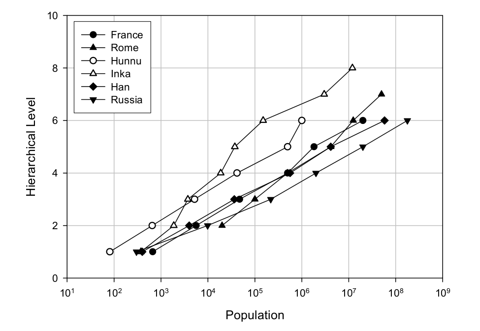Figure 12: Hierarchical level vs. population of six historical empires.
Note: Hierarchical level is counted in terms of the number of distinct administrative levels. Source: Turchin and Gavrilets (2009).

---

Logarithmic scaling (between group size and the number of administrative levels) is a predictable result of group size expansion under a fixed span of control. For any hierarchical group with a fixed span of control, the total number of members (n) can be expressed as a geometric series of the span of control (s). If L represents the number of hierarchical levels (and assuming the top level contains one person), then the total number of group members is equal to:

n = 1 +s+ s^2+s^3 + \ldots + s^{L-1}
(10)

Using the formula for the sum of a geometric series, this can rewritten as:

n = \frac{1-s^L}{1-s}
(11)

As a rough estimate, we can simplify equation 11 to equation 12, which indicates that the number of group members varies exponentially with the number of hierarchical levels.

n \sim s^{L-1}
(12)

Equation 12, in turn, can be rearranged to equation 13, which indicates that the number of hierarchical levels varies approximately logarithmically with the number of group members.

L \sim \log (n)
(13)

This logarithmic scaling appears to be robust across space and time. In the modern era, John Child (1973) finds a logarithmic scaling between modern corporation employment size and the number of hierarchical levels (Fig. 13). Hierarchy, it seems, plays an essential (and predictable) role in organizing large groups of humans. Indeed, one is hard-pressed to find an example of a large organization that exists without any hierarchy.

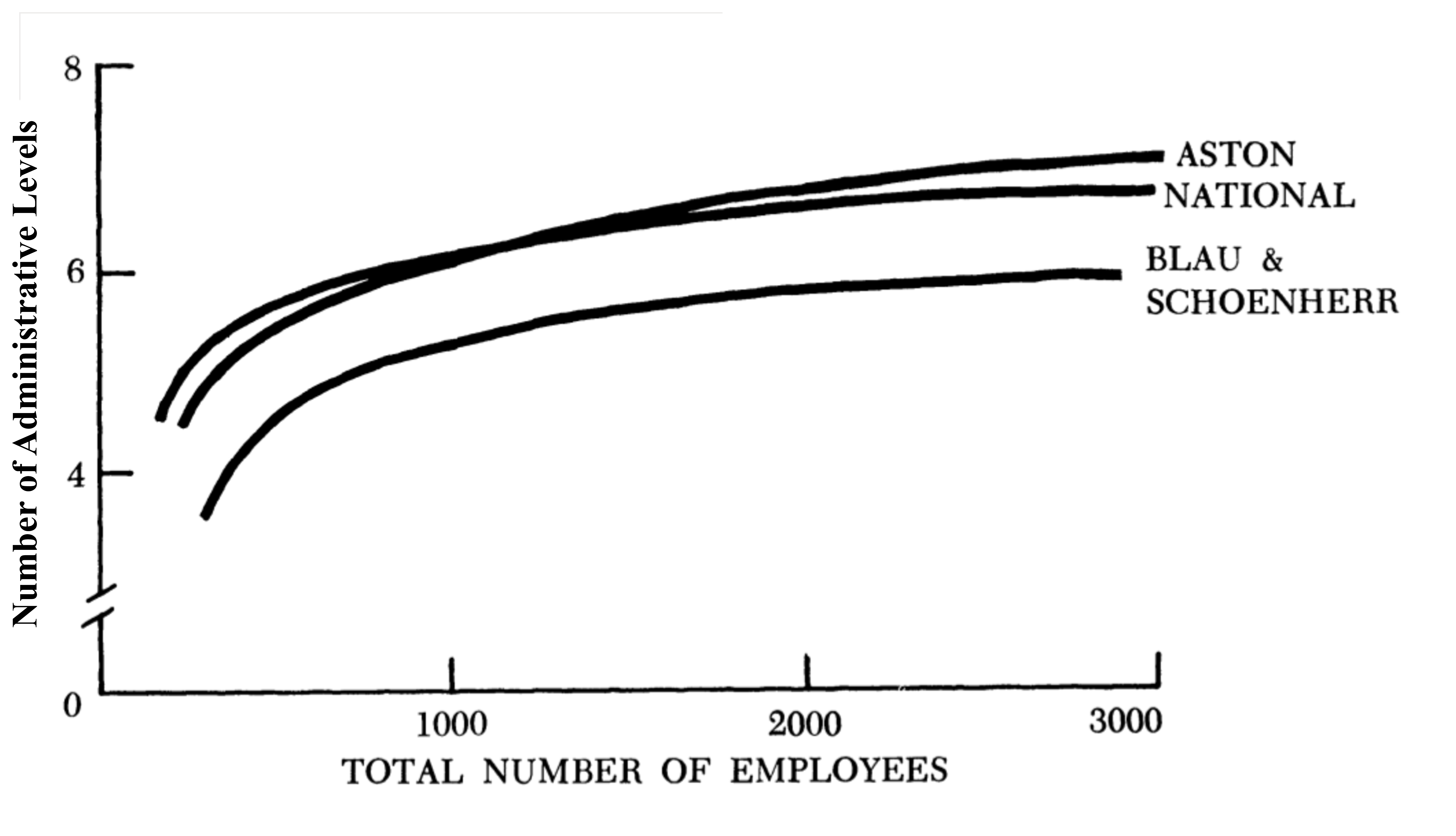Figure 13: Hierarchical levels vs. firm size.
Source: Child (1973). ‘Aston’, ‘National’ and ‘Blau & Schoenherr’ refer to different firm datasets.

---

Given the link between increases in corporate employment concentration and the growth of energy consumption, a reasonable hypothesis is that growth requires the coordination of ever-increasing swathes of humanity, and that hierarchy is the path of least resistance for such coordination.

Profit as the Fountain Head of Authority

All hierarchical institutions must have systems for legitimizing the authority of superiors and rationalizing the subservience of subordinates. Weber (1958) divided legitimization strategies into three categories: charismatic authority, traditional authority, and legal authority. Of these three, charismatic authority is by far the least stable, since there is no mechanism for transferring authority after the death of the leader.

Traditional authority is usually associated with feudal systems, or any hierarchical system based on birthright. Such systems often have elaborate ideologies for rationalizing inherited authority. Peter Turchin (2010) argues that it is not coincidental that the major world religions and the first large empires emerged during the same era (the Axial Age, 800—200 BC); religion is highly effective at legitimizing authority. By appealing to God as the source of their power, the kings of antiquity gained access to a potent ideological tool for legitimizing their authority.

According to Weber, the modern era is different from all other eras in that the rule of law has become the dominant mode of authority. Under such a system, authority has little or nothing to do with the characteristics of the ruler or his family lineage, but is instead based on a system of law that is (ideally) applied uniformly to all people. Still, laws must stem from a core belief system.

Nitzan and Bichler argue that the kernel of the modern nomos is a pervasive belief in the principle of capitalization: the belief that anything that can be ‘owned’ may be reduced to a single, abstract quantity of money. Nitzan and Bichler note:

Faith in the principle of capitalization now has more followers than all of the world’s religions combined. It is accepted everywhere — from New York and London to Beijing and Teheran. In fact, the belief has spread so widely that it is now used regularly to discount not only capitalist income, but also the income of wage earners, governments, and, indeed, society at large.

(Nitzan & Bichler, 2009, p. 8)

Capitalization allows a systematic way of defining reciprocity: if prices are equivalent, an ownership exchange is culturally defined as being reciprocal (Hornborg, 1992). In a capitalist society, hierarchical relations are rationalized by appealing to the reciprocity of monetary transactions. We all accept that the owner of a business enterprise is the rightful ‘ruler’ of his employees. Why is his authority legitimate? Because he exchanged money for ownership.

As Nitzan and Bichler note, by investing his money, the capitalist gains culturally sanctioned power to mobilize and control human labor. Importantly, this power appears (to the participants) as a reciprocal exchange, because it is wielded through a monetary transaction. This veil of reciprocity is illustrated by the terminology used: while military leaders command, capitalists invest.¹⁷

Thus, capital is a potent tool for legitimizing authority and facilitating the growth of large hierarchies. The steps that lead to this authority are similar (in principle) to those that lead to the divine authority of kings:

Divine Kingship

1. God is the ultimate authority.

2. Kings are ordained by God.

3. Kings are legitimate holders of power.

Capitalization

1. Monetary exchange is reciprocal.

2. Capitalists exchange money (capital) for ‘ownership’.

3. Owners are legitimate holders of power.

However, unlike other forms of authority, capital has a finite magnitude that is depleted when power is wielded. This presents a problem: unless capital can be renewed, it will be an ephemeral source of power. Thus, a return on the investment of capital is a fundamental requirement of capitalist authority: it allows the potential for authority to become self-renewing.

This return on investment can be realized either through interest or profit. However, for the process of hierarchy formation, the evidence suggests that profit is key. Why is this the case? It could be because profit is associated with equity, and ownership of equity gives direct command of the corporate hierarchy. Interest, on the other hand, is associated with corporate bonds, which do not give the bond-holder any say in corporate decision-making. While this is a plausible explanation, I leave a more in-depth investigation for future research.

Whatever the reason for the primacy of profit in hierarchy formation, based on the evidence in this paper, I propose the following three-way linkage between profit, hierarchy and growth:

1. The expansion of hierarchy is necessary for growth.

2. Hierarchy formation is legitimized by the investment of capital.

3. Capital accumulation, through profit, acts as a fountain head of legitimacy, allowing further expansion of hierarchy.

4. The expansion of hierarchy drives growth.

Conclusions

The evidence discussed in this paper is fundamentally at odds with the assumptions made by neoclassical growth theory: both distribution and large institutions (concentrated power) play a central role in growth. Thus, any growth theory that wishes to explain reality must begin by discarding neoclassical principles.

The theory that I have advanced draws heavily on Nitzan and Bichler’s Capital as Power framework, which is unique in political economy in that it asserts that capital is unproductive. Nitzan and Bichler conceive of capital as a form of power derived from the legal right to strategically limit production. But this leads to a paradox: if capital is unproductive, why has the capitalist era witnessed the most stupendous period of growth in the history of humanity (1800 to the present). How do we resolve this paradox?

Nitzan and Bichler are correct to assert that capital accumulation has little to do with productivity. Based on thermodynamic principles, we must insist that productivity stems from the transformation of energy. The role of physical capital (I prefer the term technomass) is to facilitate energy transformation into forms usable by humans (think of the tractor converting fossil fuels into mechanical work). However, we should not conflate technomass with financial capital (or simply capital). The latter is a quantitative abstraction that cannot be productive, by virtue of its non-physical existence.

Nitzan and Bichler argue that modern corporations are megamachines — Lewis Mumford’s (1970) term for large hierarchical organizations that function as machines by using humans as components. I argue that capital is a potent tool for facilitating the growth of such megamachines — much more potent than appeals to the divine. Because belief in the reciprocity of monetary transactions is nearly universal, capital investment legitimizes the authority of those at the top of the corporate megamachine. It is the expansion of the corporate megamachine that then drives growth. Capital accumulation thus plays a role in growth by allowing capitalists to organize vast pools of human labor, but it must be stressed that capital serves an ideological purpose, not a physical one: it veils power under the guise of monetary reciprocity.

But — and this is key — hierarchy formation seems only to occur under capital accumulation through profit (not interest). I have hypothesized that this is because profit flows to those actually in command of corporate hierarchies, while interest is passive income. The balance between profit and interest seems to determine whether employment is added in large versus atomistic institutions, and this employment balance is then related to the rate of growth.

Many questions arise from this provocative reformulation of growth theory. Perhaps most importantly, will the empirical linkages between profit, hierarchy, and growth continue into the future? How will energy limits (due to the inherent finite nature of fossil fuels) affect this linkage? Will the capitalist mode of power be viable in a ‘degrowth’ (negative growth) future? Such questions ought to be at the center of a power-based theory of growth.

Notes

References

Acemoglu, D. (2008). Introduction to modern economic growth. Princeton, NJ: Princeton University Press.
Ayres, R. U., & Warr, B. (2010). The economic growth engine: How energy and work drive material prosperity. Cheltenham, UK: Edward Elgar Publishing.
Ayres, R., & Warr, B. (2005). Accounting for growth: The role of physical work. Structural Change and Economic Dynamics, 16(2), 181–209.
Brennan, J. (2012). A shrinking universe: How concentrated corporate power is shaping income inequality in Canada. Canadian Centre for Policy Alternatives.
Bureau of Labor Statistics. (2010). Frequently asked questions about hedonic quality adjustment in the cpi. http://www.bls.gov/cpi/cpihqaqanda.htm
Chaisson, E. (2002). Cosmic evolution: The rise of complexity in nature. Cambridge, Mass.: Harvard University Press.
Child, J. (1973). Predicting and understanding organization structure. Administrative Science Quarterly, 18(2), 168–185.
Cleveland, C. J., Costanza, R., Hall, C. A., & Kaufmann, R. (1984). Energy and the US economy: A biophysical perspective. Science, 225(4665), 890–897.
Cleveland, C., Kaufmann, R., & Stern, D. (2000). Aggregation and the role of energy in the economy. Ecological Economics, 32(2), 301–318.
Coase, R. H. (1937). The nature of the firm. Economica, 4(16), 386–405.
Cobb, C. W., & Douglas, P. H. (1928). A theory of production. The American Economic Review, 18(1), 139–165.
Cochrane, D. (2011). Castoriadis, veblen, and the “power theory of capital” (I. Straume & J. Humphreys, Eds.). http://www.academia.edu/download/30846400/cochrane_2011_castoriadis_veblen_and_the_power_theory_of_capital.pdf
Cottrell, F. (2009). Energy & society (revised): The relation between energy, social change, and economic development. Bloomington: AuthorHouse.
Debeir, J. (1991). In the servitude of power: Energy and civilization through the ages. Atlantic Highlands, N.J.: Zed Books.
Dunbar, R. I. (1992). Neocortex size as a constraint on group size in primates. Journal of Human Evolution, 22(6), 469–493.
Dunbar, R. I. (1993). Coevolution of neocortical size, group size and language in humans. Behavioral and Brain Sciences, 16(04), 681–694.
Felipe, J., & Fisher, F. M. (2003). Aggregation in production functions: What applied economists should know. Metroeconomica, 54(2–3), 208–262.
Felipe, J., & Holz, C. A. (2001). Why do aggregate production functions work? Fisher’s simulations, Shaikh’s identity and some new results. International Review of Applied Economics, 15(3), 261–285.
Fisher, F. M. (1969). The existence of aggregate production functions. Econometrica: Journal of the Econometric Society, 553–577.
Garrett, T. J. (2012). No way out? The double-bind in seeking global prosperity alongside mitigated climate change. Earth System Dynamics, 3(1), 1–17. https://doi.org/10.5194/esd-3-1-2012
Georgescu-Roegen, N. (1971). The entropy law and the economic process. Cambridge, MA: Harvard University Press.
Giampietro, M., Mayumi, K., & Sorman, A. (2013). Energy analysis for a sustainable future: Multi-scale integrated analysis of societal and ecosystem metabolism. New York: Routledge.
Hall, C., & Klitgaard, K. (2012). Energy and the wealth of nations: Understanding the biophysical economy. New York: Springer.
Hirsch, R. (2008). Mitigation of maximum world oil production: Shortage scenarios. Energy Policy, 36(2), 881–889.
Hornborg, A. (1992). Machine fetishism, value, and the image of unlimited good: Towards a thermodynamics of imperialism. Man, 1–18.
Kaldor, N. (1957). A model of economic growth. The Economic Journal, 67(268), 591–624.
Keen, S. (2001). Debunking economics: The naked emperor of the social sciences. New York: Zed Books.
Kondepudi, D., & Prigogine, I. (1998). Modern thermodynamics: From heat engines to dissipative structures. Chichester: John Wiley & Sons.
Lotka, A. J. (1956). Elements of mathematical biology. http://193.190.8.15/afrilib/handle/0/2666
Lydall, H. (1971). A theory of distribution and growth with economies of scale. The Economic Journal, 81(321), 91–112.
Marx, K. (1867). Capital, volume I. Harmondsworth: Penguin/New Left Review.
Marx, K. (1894). Capital, vol. III (Vol. 35). Hamburg: Verlag.
Morowitz, H., & Smith, E. (2007). Energy flow and the organization of life. Complexity, 13(1), 51–59. http://onlinelibrary.wiley.com/doi/10.1002/cplx.20191/full
Mumford, L. (1970). The myth of the machine [vol. 2], the pentagon of power. Harcourt, Brace & World.
Nitzan, J. (1992). Inflation as restructuring. A theoretical and empirical account of the US experience (PhD thesis). McGill University.
Nitzan, J., & Bichler, S. (2009). Capital as power: A study of order and creorder. New York: Routledge.
Odum, H. T. (1988). Self-organization, transformity, and information. Science, 242, 1132–1139. http://swarma.org/thesis/doc/jake_191.pdf
Polanyi, K. (1964). The great transformation. Boston: Beacon Press.
Robinson, J. (1934). Euler’s theorem and the problem of distribution. The Economic Journal, 44(175), 398–414.
Robinson, J. (1953). The production function and the theory of capital. The Review of Economic Studies, 21(2), 81–106.
Salter, J. A. (1921). Allied shipping control. New York: Oxford: At the Clarendon Press.
Samuelson, P. A. (1938). A note on the pure theory of consumer’s behaviour. Economica, 5(17), 61–71.
Schrodinger, E. (1992). What is life?: With mind and matter and autobiographical sketches. Cambridge University Press.
Shaikh, A. (1974). Laws of production and laws of algebra: The humbug production function. The Review of Economics and Statistics, 56(1), 115–120.
Shaikh, A. (2005). Nonlinear dynamics and pseudo-production functions. Eastern Economic Journal, 31(3), 447–466.
Smil, V. (1994). Energy in world history. Boulder: Westview Press.
Smith, A. (1776). An inquiry into the nature and causes of the wealth of nations. Edinburgh: A.; C. Black.
Solow, R. M. (1956). A contribution to the theory of economic growth. The Quarterly Journal of Economics, 70(1), 65–94.
Steindel, C. (1995). Chain-weighting: The new approach to measuring GDP. Current Issues in Economics and Finance, Federal Reserve Bank of New York, 1(9).
Stern, D. (2011). The role of energy in economic growth. Annals of the New York Academy of Sciences, 1219(1), 26–51.
Swan, T. W. (1956). Economic growth and capital accumulation. Economic Record, 32(2), 334–361.
Turchin, P. (2010). Warfare and the evolution of social complexity: A multilevel-selection approach. Structure and Dynamics, 4(3).
Turchin, P., & Gavrilets, S. (2009). Evolution of complex hierarchical societies. Social Evolution and History, 8(2), 167–198.
Weber, M. (1958). The three types of legitimate rule. Berkeley Publications in Society and Institutions, 4(1), 1–11.
Wicksteed, P. H. (1894). An essay on the co-ordination of the laws of distribution (1932 edition). London: London School of Economics.
Wong, S. (1978). Foundations of Paul Samuelson’s revealed preference theory. New York: Routledge.