
Reconsidering Systemic Fear
and the Stock Market
A Reply to Baines and Hager

JAMES MCMAHON
August 2021
Abstract
This article responds to Baines and Hager’s recent critique of the capital-as-power model of the stock market. Proposed by Bichler and Nitzan, this model seeks to explain how financial crises are tied to the concept of ‘systemic fear’. Bichler and Nitzan tested their initial model on US data, finding a strong correlation between capitalist power (as they measure it) and systemic fear. However, when Baines and Hager extended the model to four other countries, they found conflicting results. I respond to Baines and Hager, and argue that they were perhaps too quick to dismiss systemic fear as a useful concept. I re-examine systemic fear in twelve countries, and find that (with a few exceptions), it correlates with capitalist power. These results suggest that the notion of ‘systemic fear’ is useful for studying both capitalist crisis and national diversity in capitalist development.
Keywords
capitalization, comparative political economy, crisis, power index, stock market, strategic sabotage, systemic fear
Citation
McMahon, James. 2021. ‘Reconsidering Systemic Fear and the Stock Market: A Reply to Baines and Hager’. Review of Capital as Power, Vol. 2, No. 1, pp. 30-70.

1 Introduction
Arecent New Political Economy article by Joseph Baines and Sandy Hager (2020) critiques Shimshon Bichler and Jonathan Nitzan’s capital-as-power (CasP) model of the stock market (Bichler & Nitzan, 2016). Bichler and Nitzan’s model seeks to explain how financial crises are tied to the (upper) limits of redistributing income through power. Their model uses American financial data to show that ‘US-based capitalists’ have risen to a great height of capitalized power relative to the underlying population. This height also produces a ‘forward-looking’ fear about the ability to accumulate even more (Bichler & Nitzan, 2016).1
Baines and Hager examine the CasP model with the financial data of four other countries:
- France
- Germany
- Great Britain
- Japan
With a careful, step-by-step approach, Baines and Hager identify where these countries have similar patterns to the United States and where they do not. Overall, Baines and Hager are concerned with the national differences in the CasP model, as they are curious to know how the CasP model of the stock market can function as a general model of capital accumulation at an international level. Based on their findings, they argue that the CasP model of the stock market is likely not suited to analyze (Baines & Hager, 2020, p. 137).
Baines and Hager’s article is rich with details and will surely stimulate future research and dialogue in political economy. My paper responds only to a specific aspect of Baines and Hager’s paper. In Section 4 of their NPE article, Baines and Hager examine Bichler and Nitzan’s concept of systemic fear, which is applied to the stock markets of the countries listed above. Bichler and Nitzan created this concept to theorize the effects of capitalists reaching limits in accumulating power.
Systemic fear is low, Bichler and Nitzan theorize, when capitalist power is low. Their reasoning:
[T]he lower the capitalized power, the greater the scope for increasing it further: income can be further redistributed in favour of profit, hype can be further amplified, profit volatility can be further decreased and the normal rate of return can be further lowered.
(Bichler & Nitzan, 2016 italics in original, p. 143)
Systemic fear rises with rising capitalist power, Bichler and Nitzan continue, because (Bichler & Nitzan, 2016, p. 143). As more things are done to increase power, such as decreasing profit volatility, it becomes harder to go even further in the interest of power. When power is already high, resistance from below grows and capitalists do not see the future as an open frontier of opportunity. In this state, systemic fear is the other side of high capitalist confidence: the and (Bichler & Nitzan, 2016, p. 142).
In their response, Baines and Hager follow the methods of Bichler and Nitzan and produce metrics of systemic fear for France, Germany, Great Britain and Japan. As an empirical metric, systemic fear measures a moving correlation between past earnings and stock prices. Note that this differs from conventional finance, which claims capitalists should be forward-looking.
The systemic fear index is produced in the following two steps (illustrated in Figure 1):
-
Calculate a 12-month trailing correlation between prices and earnings. (In the short term this trailing correlation bounces up and down between 1 and -1.)
-
Take a longer-term moving average of this trailing correlation. This transformation of the time series reveals the annual (or even decennial) trends in the correlation between prices and earnings.
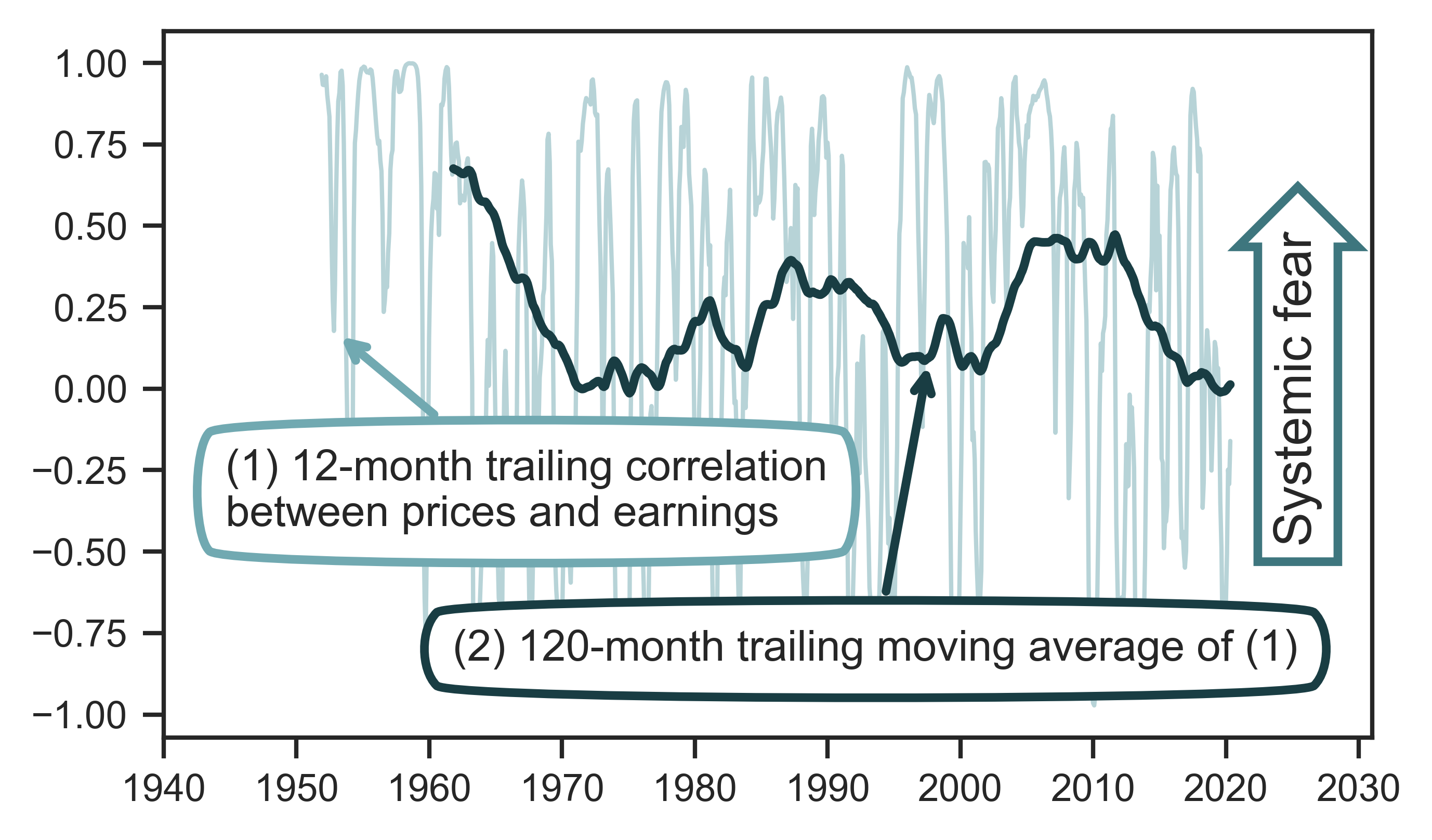
Figure 1: Constructing the systemic fear index
Note: Using data from the United Kingdom, this figure illustrates the construction of the systemic fear index. It involves 2 steps. In step 1, we compute the 12-month trailing correlation between prices and earnings (light-blue line). In step 2, we take this correlation (which varies widely over time) and compute the 120-month trailing moving average. The result is a time series of systemic fear (dark-blue line).
Sources and methods: See Table 2 for the creation of the systemic fear index. See Tables 5 and 6 for breakdown of United Kingdom data.
Having calculated Bichler and Nitzan’s systemic fear index, Baines and Hager are skeptical that, across the world, (Baines & Hager, 2020, p. 124). They recognize the strong results in the case of the United States, but see concerning differences elsewhere. For example, they conclude that Germany is the only country in their group to have a strong correlation between systemic fear and Bichler and Nitzan’s ‘power index.’2
This power index is a measure of capitalists’ relative power. As Bichler and Nitzan define it, the power index is the ratio of a stock index price (such as the S&P 500) to the average wage rate:
\displaystyle \text{power index} = \frac{\text{stock market index}}{\text{average wage rate}}
(1)
The assumption here is that stock market prices reveal capitalists’ power to earn income. Hence the power index quantifies how capitalists (who have significant stakes in the stock market) succeed or fail relative to the underlying population (who primarily rely on wage income). Based on evidence from the United States, Bichler and Nitzan argue that ‘systemic fear’ is the dialectical ‘other’ of the power index. Significant increases in the power index produce systemic fear, as in the future it is increasingly difficult to see further growth of capitalist power.
I focus my attention on the ‘systemic fear’ part of Baines and Hager’s article for two reasons. First, Baines and Hager correctly identify systemic fear to be a distinguishing feature of Bichler and Nitzan’s writings on capitalist crisis. Systemic fear signals a breakdown in the forward-looking ritual of capitalization, which discounts future expectations to present prices. Bichler and Nitzan argue that this form of breakdown is very significant because capitalization :
Suppose for argument’s sake that capitalists, instead of expecting capitalization to continue indefinitely, believed that the process would cease to exist at some future point. At that point, with capitalization gone, their assets would have a nil value, by definition; and with future prices being zero, current prices would have nowhere to trend but down. Now, the fact that capitalists invest shows that they expect the very opposite — i.e., that the value of their assets will grow, not contract — and that expectation means that, consciously or not, they also think that the ritual that valuates their assets will never end.
(Bichler & Nitzan, 2016)
Second, Baines and Hager’s analysis of systemic fear is where, in my opinion, they overlook opportunities to investigate and experiment within the CasP model. They discover cases where Bichler and Nitzan’s results do not hold, but do not further investigate why these differences exist. Instead, Baines and Hager conclude:
It may be time to move beyond systemic fear as a conceptual basis for modelling the stock market.
(Baines & Hager, 2020, p. 133)
In what follows, I discuss reasons why Baines and Hager might be too impatient with their judgment of the CasP model. The paper is broken into three sections. Section 2 summarizes how I prepared the data to engage with Baines and Hager’s critique of Bichler and Nitzan. My analysis expands the scope of previous research on the CasP model. I add more countries and create new measures of capitalist power and systemic fear. These expansions are experimental — they are done in search of more evidence, which could be used to test Bichler and Nitzan’s theory of systemic fear and its links to capitalist power.
Section 3 analyzes examples of how Baines and Hager critique the concept of systemic fear. Performing a critique is certainly not an issue on principle, but I argue that Baines and Hager are too quick in their judgment, particularly because they rely on their own definitions of ‘systemic’ and ‘crisis’ to arrive at their conclusion.
To my knowledge, Bichler and Nitzan have not presented firm opinions on how systemic fear would be measured across different stock markets. Thus, when Baines and Hager take their arguments to an international dimension, there is no body of literature to stand on — they are creating standards to analyze the international dimensions of systemic fear. This situation is what makes their article an exciting contribution to political economy. But it is also puzzling why they appear to be closing a debate that still has many unexplored paths.
Section 4 is inspired by Baines and Hager’s interest in the diversity and unevenness of capitalist development. By widening the international data, I hope to re-open the debate on the meaning of systemic fear and on the evidence of systemic fear’s relationship with capitalized power. I have three goals:
-
To experiment with the methods used to measure systemic fear and capitalist power in a way that is consistent with Bichler and Nitzan’s conceptualization of these terms.
-
To discover if, despite national differences, there is evidence of rising systemic fear at an international level.
-
To discover if, despite national differences, there is a positive correlation between systemic fear and capitalist power at an international level.
2 Data preparation
2.1 Countries and stock markets in the dataset
Hitherto, systemic fear (and its relation to capitalist power) has been analyzed in the context of national markets. To replicate Bichler and Nitzan’s measurements, I have retrieved United States data and recalculated the original index of systemic fear. To replicate the measurements of Baines and Hager, I have also calculated systemic fear for France, Germany, Japan and Great Britain. In addition to these previously studied countries, I have extended the data by calculating indices of systemic fear for Australia, Canada, Netherlands, South Africa, South Korea, Sweden and Switzerland.
Table 1 shows the geographical scope of my dataset. For details about the data underlying my measures of systemic fear and capitalist power, see Appendix.
Table 1: Countries and stock indexes used to measure capitalist power and systemic fear
| Country | Country Code | Stock Index* |
|---|---|---|
| Australia | AUS | ASX All-ordinaries |
| Canada | CAN | S&P/TSX 300 |
| Switzerland | CHE | SMI |
| Germany | DEU | CDAX |
| France | FRA | CAC All-tradable |
| United Kingdom | GBR | FTSE All-share |
| Japan | JPN | Nikkei 225 |
| South Korea | KOR | KOSPI |
| Netherlands | NLD | AEX All-share |
| Sweden | SWE | OMX Stockholm All-Share |
| United States | USA | S&P 500 Composite |
| South Africa | ZAF | FTSE/JSE All-Share |
Present-day titles of the indices are used. Global Financial Data details how each index is spliced when there are changes to the number of firms in the index. For detailed breakdown of prices, see Table 5 in Appendix. For detailed breakdown of price-earnings ratio, see Table 6 in Appendix.
2.2 Metrics of systemic fear and capitalist power
In addition to calculating the metrics of systemic fear and capitalist power proposed by Bichler and Nitzan, I introduce my own measurements of these terms. Table 2 outlines my measures of systemic fear, which I will refer to as \footnotesize S_1 , \footnotesize S_2 and \footnotesize S_3 . Table 3 outlines my measures of capitalist power which I will refer to as \footnotesize P_1 , \footnotesize P_2 and \footnotesize P_3 .
Systemic-fear index \footnotesize S_1 and power index \footnotesize P_1 are the measures introduced by Bichler and Nitzan, and replicated by Baines and Hager. The systemic-fear indices \footnotesize S_2 & \footnotesize S_3 and the power indices \footnotesize P_2 & \footnotesize P_3 are new. They are products of experimenting with the parameters and variables of systemic fear and power. When referring to the conceptual ideas behind specific measurements, I will sometimes use \footnotesize S_i to indicate a systemic fear index, and \footnotesize P_i to indicate a power index.
Table 2: Methods to produce time series of systemic fear
| Index | Correlation of … | Window | Transformations |
|---|---|---|---|
| \footnotesize S_1 | levels ( \footnotesize \text{Price} \sim \text{Earnings} ) | 12 months | 120-month trailing average |
| \footnotesize S_2 | levels ( \footnotesize \text{Price} \sim \text{Earnings} ) | 12 months | 120-month trailing average; seasonal decomposition (trend) |
| \footnotesize S_3 | 12-month differences ( \footnotesize \text{Price} \sim \text{Earnings} ) | 120 months | 12-month trailing average |
Note: The symbol ‘ \footnotesize \sim ’ represents correlation.
Sources: Global Financial Data for composite index prices and price-earnings ratio. Earnings are found in price-earnings ratio. For detailed breakdown of prices, see Table 5 in Appendix. For detailed breakdown of price-earnings ratio, see Table 6 in the Appendix.
Table 3: Methods to produce time series of power indices
| Index | Numerator | Denominator | Transformations |
|---|---|---|---|
| \footnotesize P_1 | Close Price | Wage Rate | log; series mean \footnotesize = 100 |
| \footnotesize P_2 | Close Price | Income per capita (Nominal) | log; series mean \footnotesize = 100 |
| \footnotesize P_3 | Close Price | GDP per capita (Nominal) | log; series mean \footnotesize = 100 |
Sources: Global Financial Data for composite index prices and GDP per capita. Income per capita (Nominal), for each country, from 1950 to 2018, taken from World Inequality Database (https://wid.world/). For detailed breakdown of wage rates, with data sources, see Table 8 in Appendix. For detailed breakdown of GDP per capita, see Table 6 in the Appendix.
2.3 Stock market price and earnings data
A common problem in political-economic research is that outside the United States, comprehensive financial data is difficult to find. Plagued by this problem, Baines and Hager’s non-US indices of systemic fear are relatively short in terms of historical depth. This shallowness is especially troublesome when creating an index of systemic fear. As a moving correlation between share price and earnings per share, the calculation of systemic fear is limited by the shortest series in the pair.
Through its platform ‘Finaeon’, Global Financial Data (GFD) provides a way to produce longer time series of prices and earnings for composite indices. GFD provides data for the price-earnings ratio — the ratio of stock price to earnings per share. By combining the price-earnings ratio with price data, we can solve for earnings per share:
\displaystyle \text{earnings per share} = \text{price} \times \frac{1}{\text{price-earnings ratio}}
(2)
Ideally, we could study the long-term behavior of the stock-market using raw earnings-per-share data. But lacking such data, using a price-earnings ratio to solve for earnings is an adequate workaround.
To confirm this workaround, Figure 2 shows American systemic fear, calculated with two different data sources. The thin line calculates systemic fear using Bichler and Nitzan’s original data source (updated to 2020). This dataset contains price and earnings-per-share data for the S&P 500. The darker line calculates systemic fear using the earnings-per-share workaround (Equation 2). As indicated by a near-perfect correlation, the differences between the methods are minor.
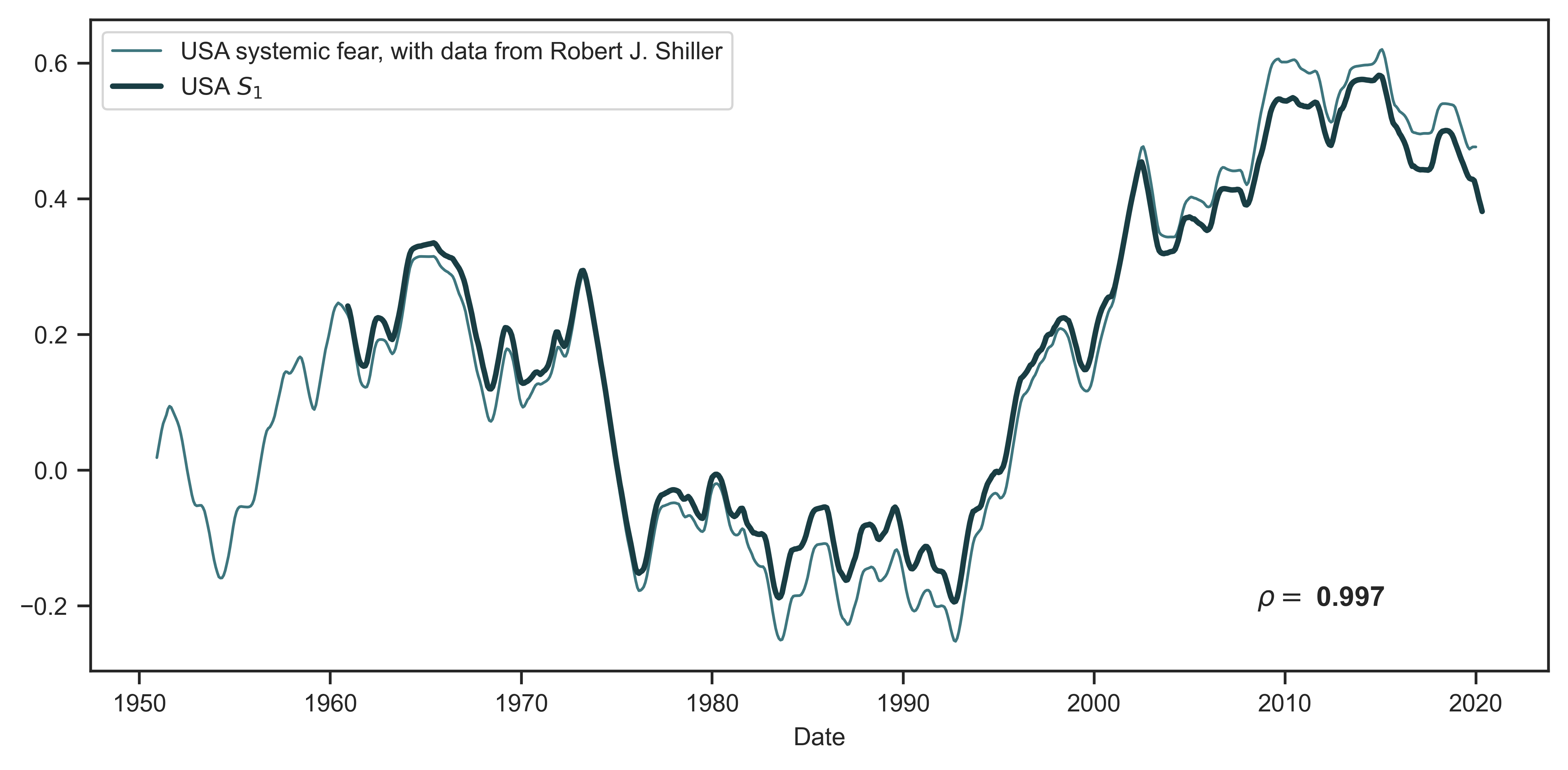
Figure 2: A systemic fear index for the United States, constructed with two different methods
Note: This figure tests the workaround of using the price-earnings ratio to construct an index of systemic fear. The thin line shows a systemic fear index constructed with Bichler and Nitzan’s original data source — data from Robert Shiller. The thick line measures systemic fear using the price-earnings ratio (Equation 2). The near identicalness of the two series indicates that the price-earnings-ratio workaround is suitably accurate.
Source and methods: Bichler and Nitzan’s measure of systemic fear calculates the rolling correlation between the price and earnings-per-share data of the S&P 500 (Bichler & Nitzan, 2016). Their data comes from Robert Shiller’s dataset (http://www.econ.yale.edu/~shiller/data/ie_data.xls, here accessed on May 19, 2020). See Table 2 for the creation of systemic-fear index \footnotesize S_1 . See Tables 5 and 6 for breakdown of United States data.
3 Baines and Hager’s critique of systemic fear
In their critique of systemic fear, Baines and Hager are (in my opinion) too quick to pass judgment on the CasP model of the stock market. While their opinion could ultimately be correct, they did not fully explore an alternative to the perceived faults in the model.3
In their analysis, Baines and Hager discovered that there are differences between the United States and other advanced capitalist countries. This fact leads them to express skepticism about the validity of the CasP model of the stock market. I contend, however, that there is room to explore the significance of these national differences. With more data, and some experimentation with how we measure Bichler and Nitzan’s concepts, we can reconsider the role of national differences in a larger model of systemic fear and capitalist power.
The remainder of this section looks at Baines and Hager’s interpretation of what makes a phenomenon ‘systemic’. From their interpretation of when and how international systemic fear should occur, Baines and Hager express skepticism when systemic fear does not behave as they think it should. For instance, they argue that systemic fear should have risen during Brexit (when it did not). And, if it is to be ‘systemic’, Baines and Hager argue that systemic fear should rise and fall collectively, across all major stock markets.
To consider whether systemic fear is indeed ‘systemic’, and to frame my analysis of Baines and Hager’s arguments, consider Figures 3 and 4. Figure 3 replicates Baines and Hager’s methods, and shows correlations between the ‘original’ systemic fear index ( \footnotesize S_1 ) and the ‘original’ power index ( \footnotesize P_1 ) for eleven countries. (The plot of South Africa is missing due to a lack of wage data, needed to calculate the power index. Extrapolating from Figure 12, the \footnotesize S_1 – \footnotesize P_1 correlation for South Africa is likely moderate but negative.)
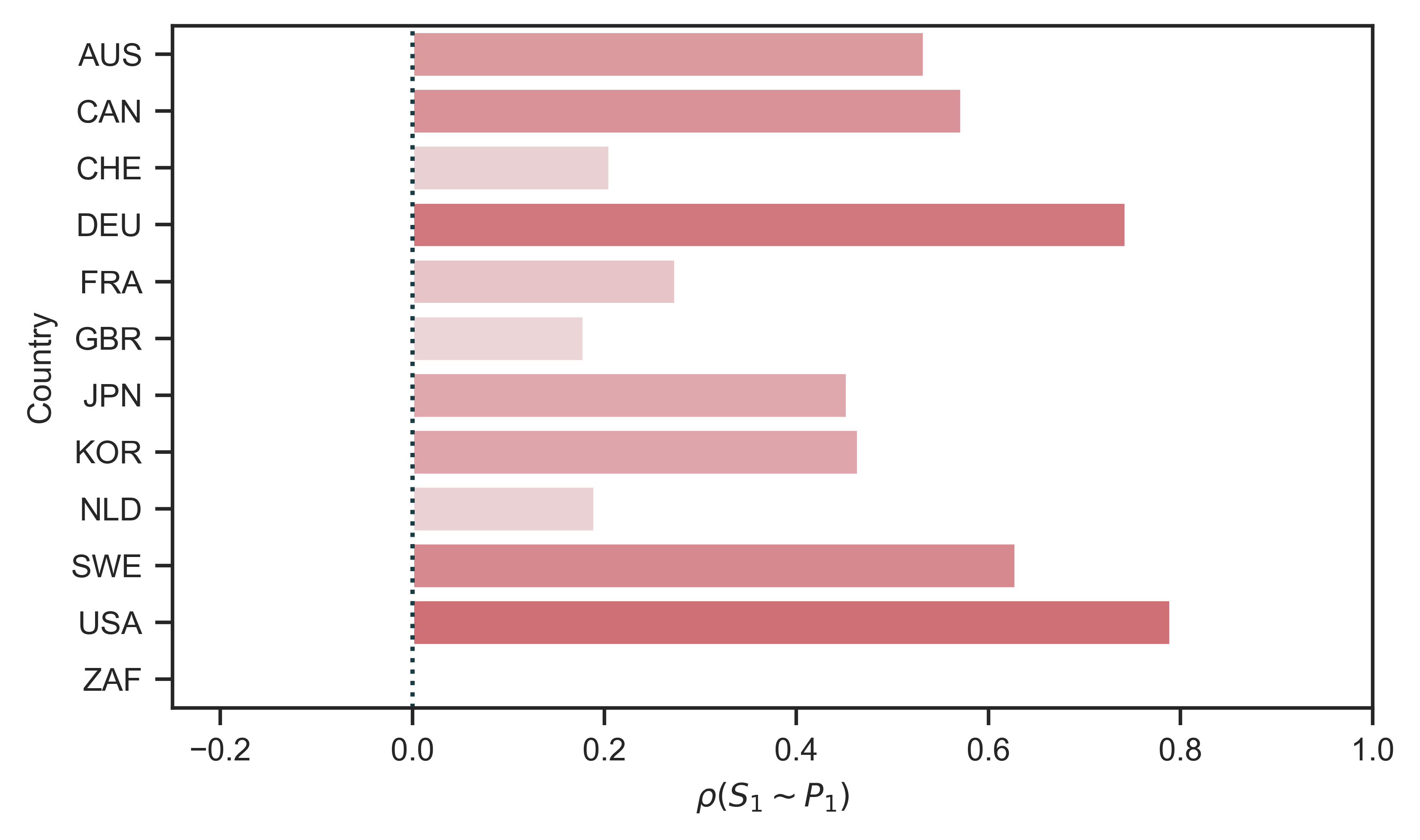
Figure 3: Country-level correlations between systemic-fear and capitalist power
Note: The vertical axis shows the 11 countries in my sample, labelled with alpha-3 codes. (South Africa is missing due to a lack of wage data, needed to construct the power index.) The horizontal axis shows the correlation between systemic-fear index \footnotesize S_1 and power index \footnotesize P_1 (the original metrics proposed by Bichler and Nitzan). In addition to the bar chart, I have used color to indicate the strength of the correlation.
Source and methods: See Table 2 for the creation of systemic-fear index \footnotesize S_1 and Table 3 for the creation of power index \footnotesize P_1 . See Appendix for breakdown of data by country.
The results in Figures 3 (which deepen the historical time frame and add more countries to the study of the CasP model of the stock market) show why Baines and Hager looked at stock markets outside the United States. The United States has the strongest positive correlation between systemic fear and capitalist power. Countries such as Germany, Canada and Sweden also have strong positive correlations. But there are weak correlations elsewhere. In particular, two of the countries first analyzed by Baines and Hager (Great Britain and France) have weak positive correlations.
In short, my extended evidence suggests that Baines and Hager were correct to conclude that the relation between capitalist power and systemic fear varies by country. But does that mean that systemic fear is not ‘systemic’? Figure 4 casts doubt on such a judgment. I have plotted here three measures of average systemic fear. (See Table 2 for the definition of each metric.) The blue line shows average systemic fear across my sample of countries. The shaded region shows the standard deviation of systemic fear.
In Figure 4, two findings are important. First, average systemic fear has long-term patterns — something we would not expect if systemic-fear trends between countries were unrelated. Second, from the late 1970s onward, average systemic fear appears to be rising.4 These results hint that systemic fear is indeed ‘systemic’, meaning capitalists in developed nations co-experience fear.
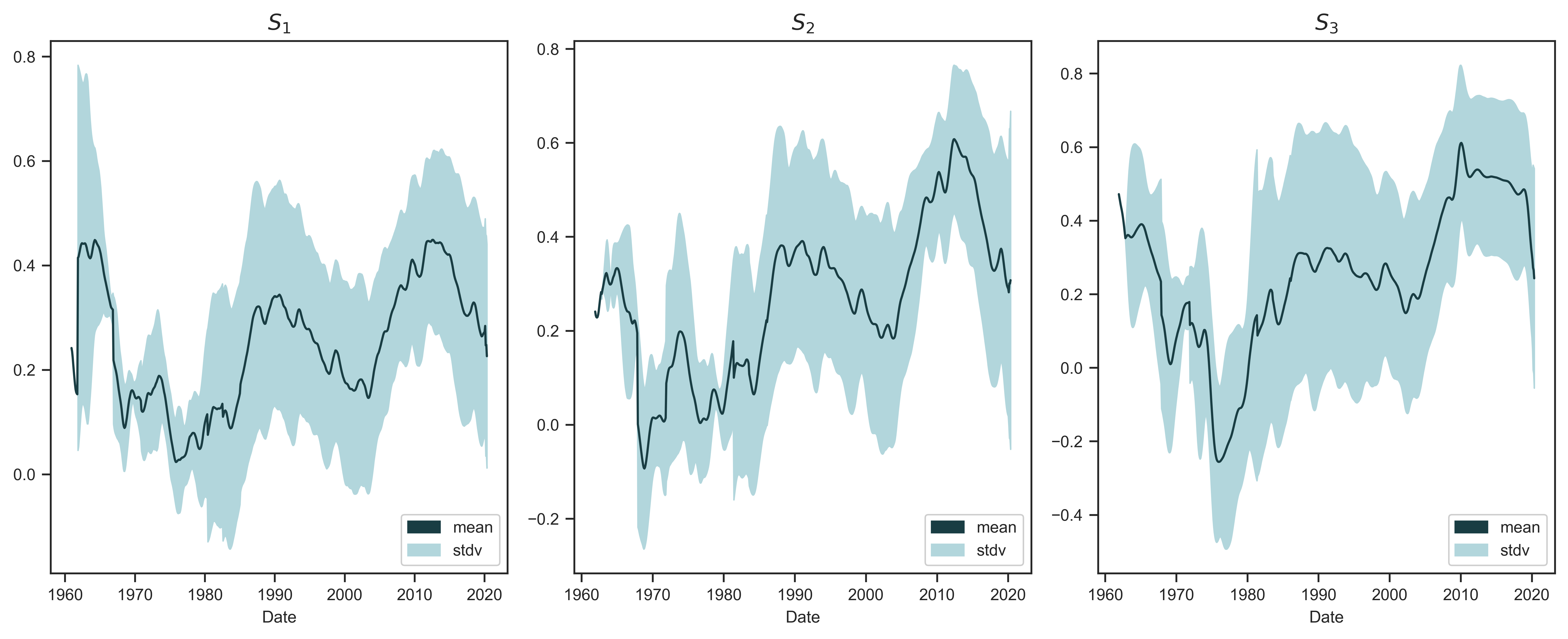
Figure 4: International averages of systemic fear
Note: Each panel shows a different measure of systemic fear ( \footnotesize S_1 , \footnotesize S_2 and \footnotesize S_3 ). See Table 2 for their definition. To produce the trend line in each panel, I take the unweighted average of systemic fear across the 12 countries in my sample. The shaded region indicates the standard deviation across countries.
Source and methods: See Table 2 for the creation of systemic-fear indices \footnotesize S_1 , \footnotesize S_2 and \footnotesize S_3 . See Appendix for breakdown of data by country.
A note about Figure 4: Empirically, each observation comes from a country, but country labels are meaningless when the sample means and standard deviations are produced by identically and independently drawing observations from the same underlying distribution of data. Thus, there can be differences in the independent events of systemic fear (e.g., the systemic fear of the United States or France), and some of these events can even be trending downwards; but the ‘expected’ outcome, based on the average, has been rising since the late 1970s.5
3.1 What does it mean for systemic fear to be ‘systemic’?
Baines and Hager argue that, by its very definition, ‘systemic’ fear should be evident at a global scale. Yet in their assessment, it is not:
… if capitalist fear is systemic, then it should be global given the integrated nature of the world’s financial system. That is to say, the strong correlation between EPS and stock prices that BN find in the US over recent years should also be evident in the major stock markets the world over. In our own research, however, we find little evidence of systemic fear as a global affliction.
(Baines & Hager, 2020, p. 131)
The premise of Baines and Hager’s critique makes sense, given the assumption that global finance is an integrated system of markets. Yet notice that Baines and Hager do not provide clear standards for labeling processes ‘systemic’. To be ‘systemic’, how many countries need to have a strong correlation (between systemic fear and capitalist power) like that of the United States? To have international ‘systemic’ fear, does every observation (of \footnotesize S_1 ) need to be above a certain value? Must there be a long-term average of high systemic fear? Must the systemic fear of each country move up and down together?
This paper cannot address all these questions in significant detail. But we should at least consider them. If questions like these are overlooked, we might fail to adequately assess the international relevancy of Bichler and Nitzan’s theory. Figure 3 confirms that there are national differences in the relationship between power index \footnotesize P_1 and systemic-fear index \footnotesize S_1 . But, to embody the skepticism of David (Hume, 1985), we are still missing a set of rules to determine if ‘systemic’ is a misleading term for the causes of these national differences.
For instance, the evidence indicates that multiple major stock markets behave similarly to the United States, in that their systemic fear correlates strongly with capitalist power: Germany ( \footnotesize +0.74 ), Sweden ( \footnotesize +0.63 ), Canada ( \footnotesize +0.57 ), and Australia ( \footnotesize +0.53 ). If we include countries that have positive correlations greater than \footnotesize +0.40 (a common benchmark for a moderate relationship between variables), we could add Japan and Korea to this list.
We certainly cannot ignore the weaker correlations either. For instance, Great Britain’s weak correlation between systemic fear and capitalist power ( \footnotesize +0.18 ) is curious, to say the least. Great Britain has one of the largest stock markets on the planet, and the country is a common subject of political-economic research. But it is still not easy to say its weak positive correlation (shown in Figure 3) is a clear sign that ‘systemic’ is an inappropriate term to describe stock-market behavior.
For comparison, take a phenomenon like air pollution. A standard measure of air quality is ‘PM2.5’, which looks at exposure levels to particulate matter that is smaller than 2.5 micrograms. One does not successfully dispute that air pollution is a ‘systemic’ problem if he states that, in recent years, many countries have exposure levels that are fractions of the levels found in the most polluted places. Successful arguments for (or against) a theory of ‘systemic’ air pollution must involve creating methods to interpret the distribution of data and the time correlations between countries — including the countries that have relatively low levels of air pollution.
To think more about the international distribution of systemic fear, we can study three characteristics of the evidence:
-
the correlation between the systemic fear of different countries;
-
the rarity of systemic fear;
-
the statistical significance of systemic fear’s distribution.
While these criteria are not the only relevant characteristics of systemic fear, knowing more about them enables us to judge whether systemic fear is (or is not) ‘systemic’, given that the data is not uniform across countries.
3.2 Trends in systemic fear: correlations between countries
In Figure 3 of their NPE paper, Baines and Hager look at the relation between systemic fear in the United States and trends in global systemic fear, calculated using the MSCI World Index (an index of global stock-market performance). Baines and Hager identify two qualities of interest:
-
the two series are positively correlated in the long term ( \footnotesize +0.59 );
-
the two series diverge in the years following the 2008 global financial crisis.
Note that missing from this comparison of the two series is a breakdown of which countries contribute to the positive correlation and which do not. Any or all countries other than the United States could be responsible for the post-2008 divergence of the United States and the MSCI index.
Furthermore, the MSCI World Index is a composite index that is weighted by shares. According to a May 29, 2020 fact sheet (MSCI, 2020), the index had the weights shown in Table 4. Given the dominance of US data in the MSCI index, the long-term positive correlation between the MSCI systemic-fear index and the US systemic-fear index could be caused by auto-correlation — the US stock market correlating with itself.6
| Country | MSCI Weight |
|---|---|
| United States | 65.8% |
| Japan | 8.2% |
| United Kingdom | 4.5% |
| France | 3.3% |
| Switzerland | 3.2% |
| Other | 14.9% |
To untangle this problem, Figure 5 shows the correlation matrix of how each country’s systemic fear (series \footnotesize S_1 ) correlates with the systemic fear of every other country in my dataset. Across each row and down each column are the pairings of two countries. The boxes show the associated correlation for trends in systemic fear. In addition to the table of correlation values, I have used color to indicate the strength of the correlation. (Red indicates a stronger positive correlation. Blue indicates a stronger negative correlation.)
The positive correlations in Figure 5 are neither perfect nor uniformly distributed across samples. Yet the results indicate that many of the countries in my sample have trends in systemic fear that positively correlate with each other. Additionally, some of these positive correlations are stronger than \footnotesize +0.59 , the value in Figure 3 of (Baines & Hager, 2020).7
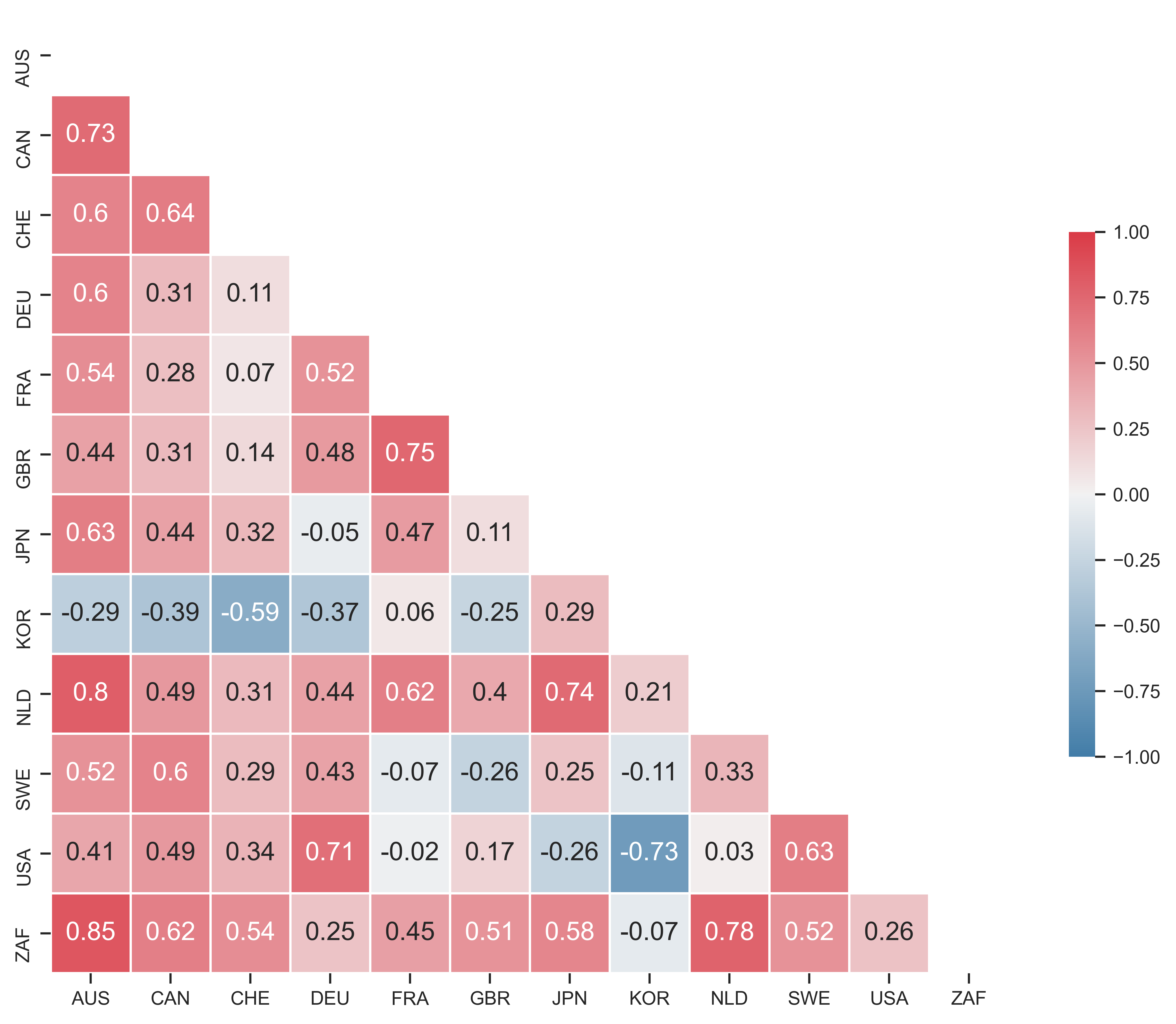
Figure 5: Correlation between countries in the trends in systemic fear
Note: In this ‘correlation matrix’, each square shows the correlation (over time) in the systemic-fear index \footnotesize S_1 between two countries. The country pairings are shown on the horizontal and vertical axis. Color indicates the strength of the correlation. (Red indicates a stronger positive correlation. Blue indicates a stronger negative correlation.)
Source and methods: See Table 2 for the creation of systemic-fear index \footnotesize S_1 . See Appendix for breakdown of data by country.
To move from analyzing the long-term correlations between countries to analyzing the historical timing of the divergence of US systemic fear from global systemic fear (measured with the MSCI World Index), we need a different approach. Figure 6 uses this paper’s dataset to perform a breakdown of country-to-country correlations of systemic-fear index \footnotesize S_1 . In each panel of Figure 6 we have a country. The time series is the average of that country’s 60-month correlations with every other country in the dataset. (For example, Australia’s panel would be the average of AUS- \footnotesize S_1 \footnotesize \sim CAN- \footnotesize S_1 , AUS- \footnotesize S_1 \footnotesize \sim CHE- \footnotesize S_1 , AUS- \footnotesize S_1 \footnotesize \sim DEU- \footnotesize S_1 , \footnotesize \ldots )
Figure 6 confirms what Baines and Hager were first to discover: that the 2008 global financial crisis marked a key historical change for systemic fear (series \footnotesize S_1 ). Countries that were tightly correlated with each other in the years before 2008 were only loosely correlated in the years that followed. In the cases of France, Germany, Great Britain, Switzerland, and the United States, the declines in correlation were particularly severe.
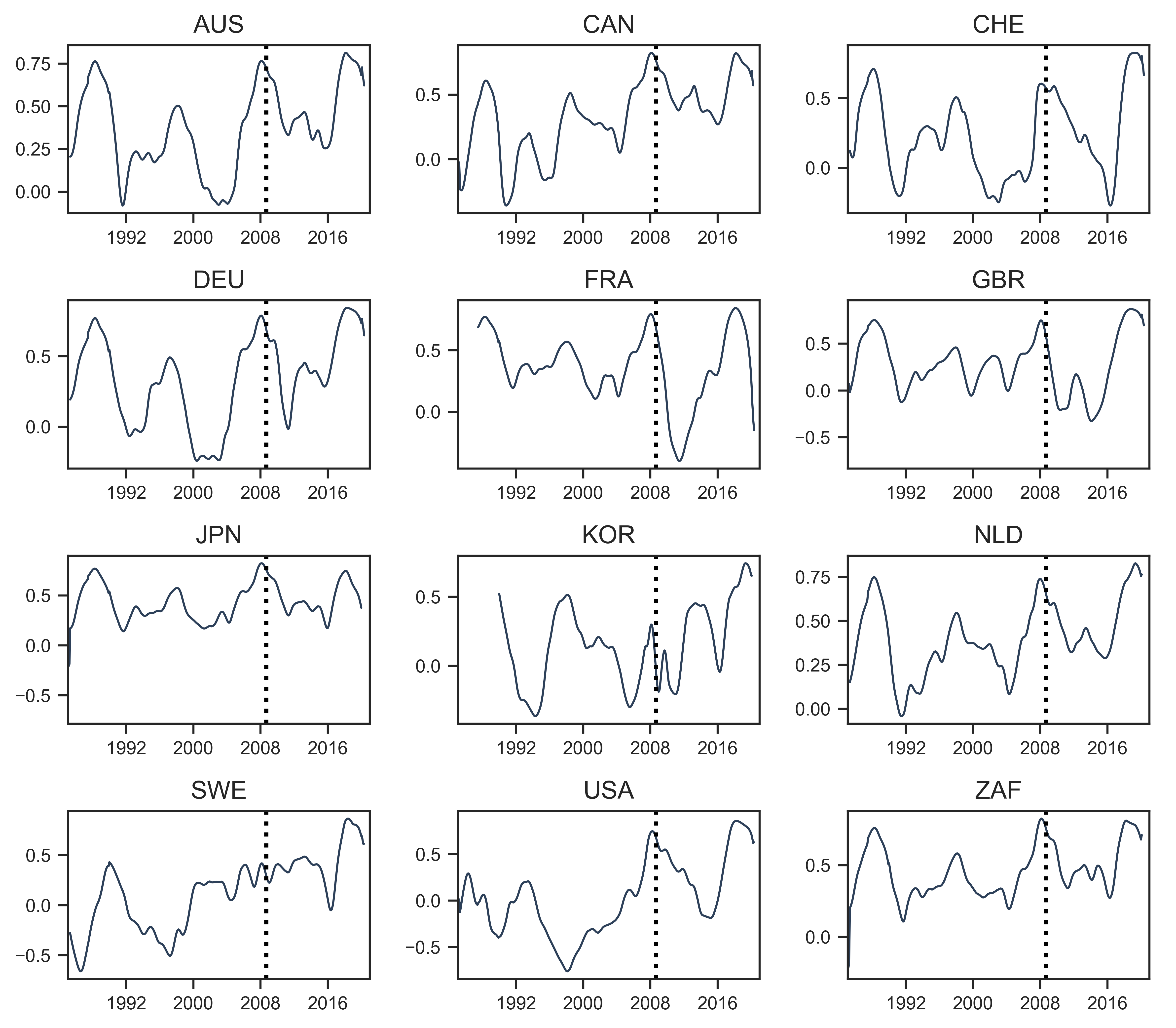
Figure 6: Changes in systemic-fear correlation across countries
Note: Each panel shows the average 60-month rolling correlation between the systemic fear index \footnotesize S_1 in the given country, and all other countries. This calculation involves 2 steps. I first calculate all possible pairings of 60-month correlations. Then for a given country, I take the average of all pairings, giving the resulting trend line. The dotted vertical line indicates the onset of the 2008 financial crisis (set here to September 7, 2008, the date of the US federal takeover of Fannie Mae and Freddie Mac).
Source and methods: See Table 2 for the creation of systemic-fear index \footnotesize S_1 . See Appendix for breakdown of data by country.
Figure 6 also suggests, however, that what has happened since 2008 is not a reason to downgrade the concept of systemic fear, but rather to look at national relationships more closely. Since the 2008 financial crisis (marked as a vertical line on the date of the US federal takeover of Fannie Mae and Freddie Mac), there is a pattern that is shared by many countries in the dataset.
After 2008, the country-to-country correlations of systemic fear (index \footnotesize S_1 ) first drops to the point where there is virtually no correlation between countries. Then, around 2016, there is a noticeable ‘bounce-back’ in the country-to-country correlations. In fact, the ‘bounce-back’ is so large that, in many cases, country-to-country correlations of systemic fear are higher today than they were in 2008. Moreover, the time series trend upwards, suggesting that the rise of average systemic fear (shown in Figure 4) is a creating stronger co-experience of fear.
3.3 The rarity of systemic fear
At particular points in recent history (such as the financial crisis of 2008 and Brexit), Baines and Hager expect that systemic fear should be rising. And yet it appears not to:
The S&P 500 systemic fear index has moved sideways at an unprecedented high from 2008 onwards, while the fear of investors in the MSCI World has plummeted over the same period. Aside from holders of S&P 500 shares, it appears, at least by BN’s measure, that capitalists the world over have been rapidly gaining confidence since the global financial crisis.
(Baines & Hager, 2020, p. 124)
Baines and Hager have expectations for systemic fear because, like many political economists, they are keen to know if a concept or method can explain key historical events. Yet it is doubtful that we know enough about international systemic fear to suggest that a particular measure of it should be moving one direction or another.
What does it mean when a measure of systemic fear tells us that ? Does it mean the measure is broken? Or does it mean that the measurement is functional, but that capitalists outside the United States are actually regaining confidence?
Answering these questions of accuracy cannot be solved quickly and it is likely that the scale of this paper is not suited to deciding whether a particular measurement of systemic fear is meaningful in every context. Yet these gaps in our knowledge affect Baines and Hager’s argument as well. Without a more detailed outline of how systemic fear relates to other crises, political or otherwise, Baines and Hager’s usage of Brexit shows signs of confirmation bias:
Perhaps the most compelling case against the systemic fear index is the fact that it has been sharply falling for the UK even in the context of the vote for Brexit in the referendum of June 2016. Other quantitative indicators of business confidence, such as the Hargreaves Lansdown Investor Confidence Index, as well as qualitative surveys of business leader sentiment, all point to a growing climate of fear in the wake of the Brexit referendum.
(Baines & Hager, 2020, p. 132)
Why must Britain’s systemic fear be high in the time of Brexit? Brexit is legitimately a front-page news story, but are the swirls of social uncertainty related to Bichler and Nitzan’s notion of systemic fear, particularly confidence in obedience?
Incompleteness of their model notwithstanding, Bichler and Nitzan delimit ‘systemic fear’ in two important ways. First, they argue that the purpose of measuring systemic fear is to estimate drops in the capitalist belief that the forward-looking logic of capitalist investment will carry into the future. Drops in this belief irritate the nervous system of the capitalist nomos, as the health of the capitalization ritual is, in the language of Castoriadis, a social imaginary signification that is (Castoriadis, 1998, p. 371).8
Second, ‘systemic fear’ is different from uncertainties that would, in the day-to-day functioning of business enterprise, be quantified as ‘risk’. As Frank H. Knight argues, we need to see the gradations and differences in economic uncertainty. Some uncertainty, for example, (Knight, 1921, p. 46). Thus, capitalists can have low expectations and still be forward-looking in behavior. In this case there would be uncertainty about the future, but the forward-looking ritual of capitalization is doing its job — these uncertainties become probabilities of future outcomes.
If we choose not to abandon the concept of systemic fear just yet, we have the opportunity to investigate how we can avoid instances of confirmation bias in the future. For example, Figure 7 plots two confidence indices from the OECD — a business confidence index (BCI) and a consumer confidence index (CCI). The time series of Great Britain are in bold. I have added time series for Germany, France and the United States for comparison. Great Britain’s consumer confidence index has dropped since 2016, but its business confidence index has been increasing with a seasonal cycle. Additionally, Great Britain’s BCI after 2016 is not visibly different than the BCIs of Germany, France and the United States.
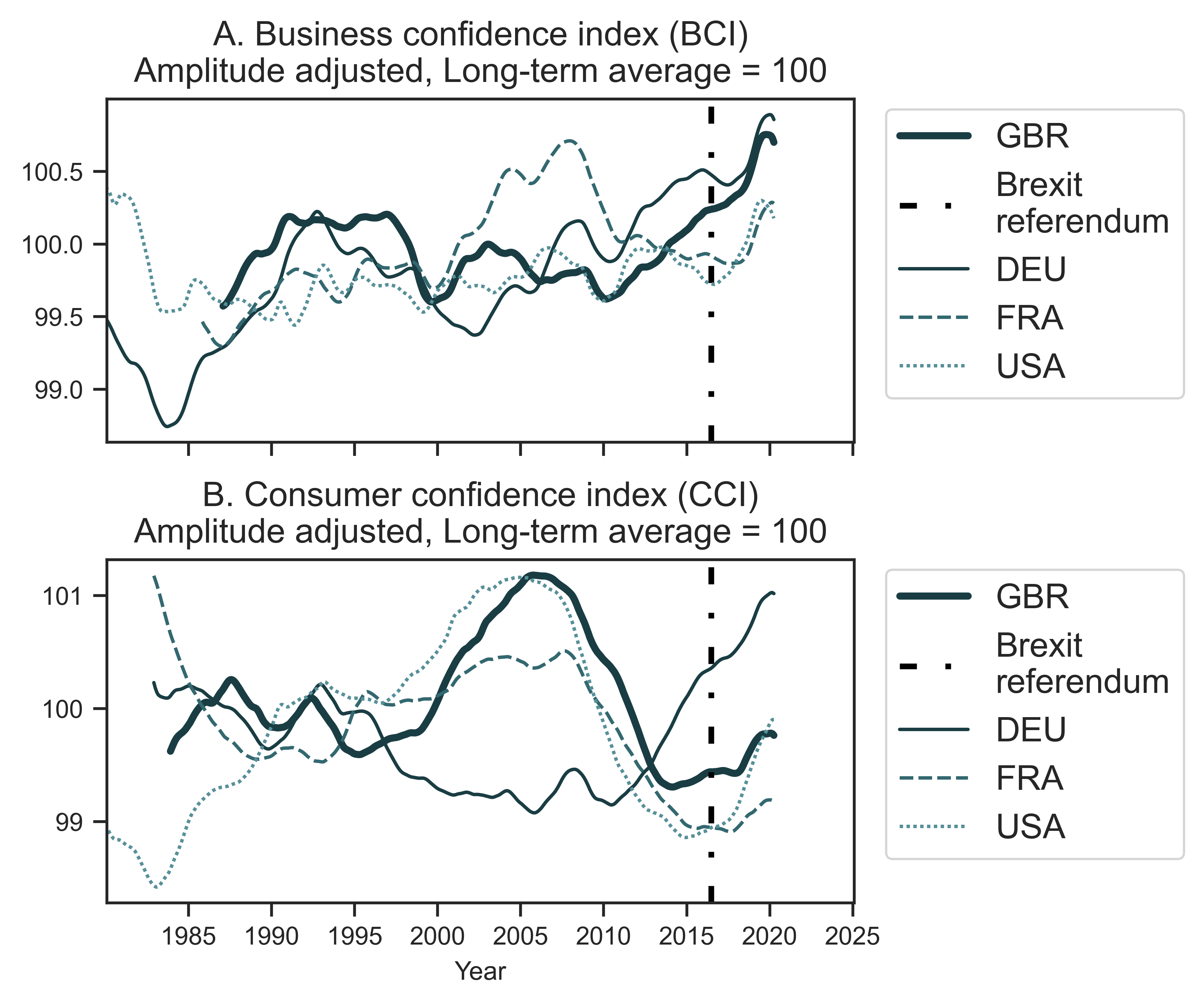
Figure 7: OECD indices of economic confidence
Note: I have plotted here two OECD measures of economic confidence: the Business Confidence Index (panel A) and the Consumer Confidence Index (panel B). I show trends for Great Britain (GBR), Germany (DEU), France (FRA) and the United States (USA). The date of the Brexit vote is marked with a dashed vertical line.
Source: OECD Main Economic Indicators: Business tendency and consumer opinion surveys: (BCI: https://data.oecd.org/leadind/business-confidence-index-bci.htm, CCI: https://data.oecd.org/leadind/business-confidence-index-bci.htm, both accessed on May 19, 2020).
This evidence in Figure 7 is a counterpoint to the way Baines and Hager use investor confidence indices. For instance, Baines and Hager argue that the Hargreaves Lansdown Investor Confidence Index shows a loss of business confidence during Brexit, while the systemic fear index indicates growing confidence. Baines and Hager therefore conclude that in the context of Brexit, Great Britain’s systemic fear ‘should’ be rising. But should it? Does the fact that systemic fear failed to rise during Brexit indicate a fatal theoretical problem with the concept itself? Because this research is preliminary, it may be too early to say.
Given that systemic fear cannot be, according to the current norms of capitalist behavior, anything like ‘everyday’ uncertainty, we should re-open the hypothesis that systemic fear is a rare state of crisis. What this means for the duration of this state, I do not know. But it does mean that we need to be just as open-minded about drops in systemic fear as we are about its rises.
We also need to investigate how systemic fear is potentially different (both theoretically and empirically) from other measures of financial confidence. Obsessed with the future, many economists, financial analysts, and journalists look for signs of economic crisis by measuring drops in economic productivity, inflated asset prices, and over-valued stock markets. Are these phenomena ‘systemic fear’ by other names?
To gain insight into this question, Figure 8 plots average 60-month correlations between systemic-fear index \footnotesize S_2 and three measures that are commonly used by investors to assess market confidence and long-term valuation:
-
The ‘Buffet indicator’: the ratio of total market capitalization to GDP. The indicator is named after Warren Buffet, who said in 2001 that (Buffett, 2001).
-
CAPE3: a three-year, cyclically-adjusted price-earnings ratio. This form of price-earnings ratio was first popularized by Robert Shiller. It measures a ratio of prices to a moving average of earnings (three years in this case). When this ratio is high, (Shiller, 2005, p. 177).
-
OECD BCI: uses opinion surveys to assess . (Note: this index was also used in Figure 7.) According to the OECD, (OECD, 2020).
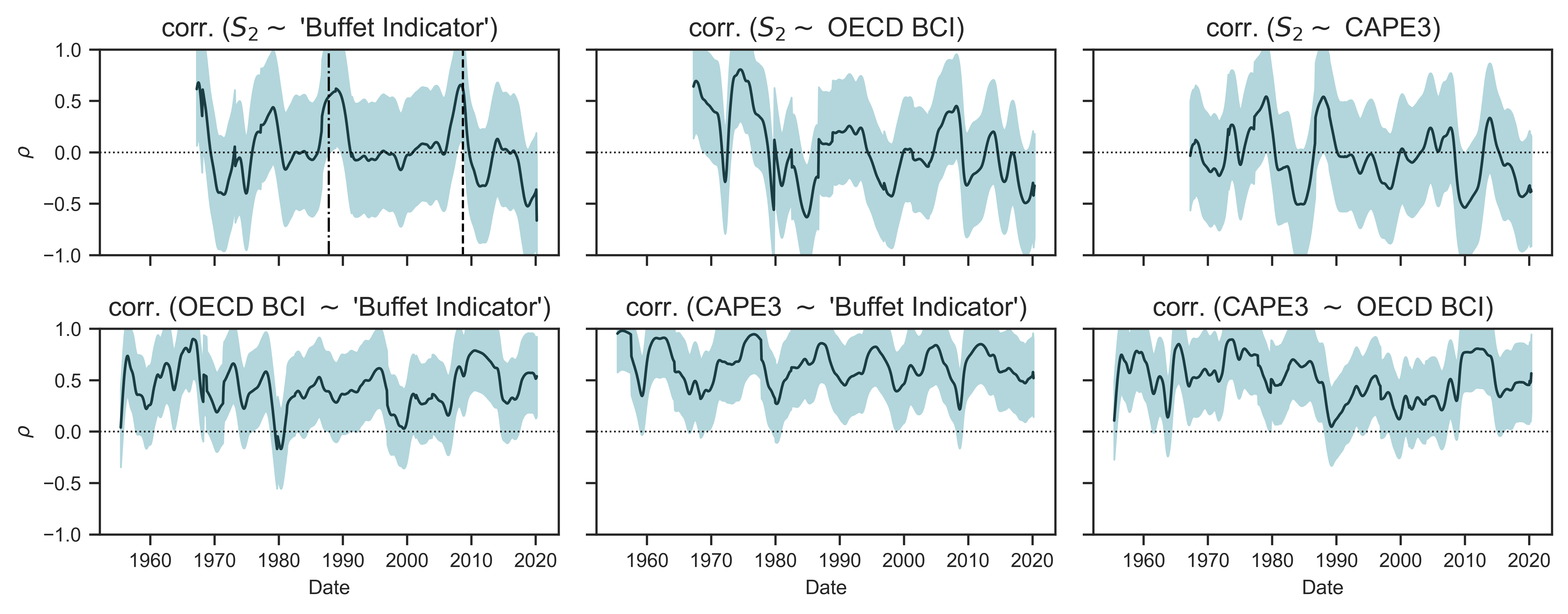
Figure 8: Rolling correlations between systemic fear (index \footnotesize S_2 ) and other indicators of business confidence
Note: The trends in this figure are calculated in 2 steps. I first calculate, for each country in my dataset, the rolling 60-month correlation between systemic-fear index \footnotesize S_2 and the given business confidence indicator. I then calculate the mean of the results, plotted as a dark line. The shade region shows the standard deviation across countries. Correlations between measures of business confidence and systemic-fear indices \footnotesize S_1 and \footnotesize S_3 yield similar results.
Source and methods: See Table 2 for the creation of systemic-fear index \footnotesize S_2 . See Appendix for breakdown of data by country. OECD BCI: https://data.oecd.org/leadind/business-confidence-index-bci.htm, accessed on May 19, 2020.
Figure 8 shows that systemic fear is often different than the other measures of investor confidence — to say nothing of differences in the theory behind these measures. Moments when systemic fear (index \footnotesize S_2 ) has a 60-month positive relationship with another measure appear to be brief and occur during bear markets.
In the top left panel of Figure 8, for example, two vertical lines show instances when the 60-month correlation between systemic fear (index \footnotesize S_2 ) and the ‘Buffet Indicator’ jumps. The first line is Black Monday (October 19, 1987). The second line is the US federal takeover of Fannie Mae and Freddie Mac (September 7, 2008), one of the many significant events at the start of the global financial crisis of 2008. By comparison, the three bottom panels in Figure 8 show that the ‘Buffet Indicator’, the CAPE3, and the BCI have positive relations throughout the market cycle.
Figure 8 cannot tell us whether systemic fear is what political economists should be looking at. Rather, the figure indicates that systemic fear (assuming it is theoretically sound) gives a different picture than other indicators of investor and business confidence. In particular, its picture of capitalist confidence after 2008 is almost the inverse of what other indicators show.
3.4 Systemic fear’s distribution
Baines and Hager observe that the systemic fear of investors in the United States (measured by the S&P 500) has moved ‘sideways’ since 2008. If one looks at Figure 2 again, one will see that this plateau occurs between the values of \footnotesize +0.40 and \footnotesize +0.60 . If we remember that a measure of systemic fear is built from a moving correlation of prices and earnings, plateauing at a ‘moderate’ level of correlation might be puzzling. What would make systemic fear approach the maximum correlation of \footnotesize +1.00 ? Is the observed maximum (of \footnotesize +0.60 ) some type of ceiling?
In addition to Baines and Hager, (Kliman, 2011) has critiqued the concept of systemic fear in reference to events in time where systemic fear, if meaningful, should be high or low.9 But nobody, to my knowledge, has investigated where ‘high’ systemic fear starts on a continuous scale. This investigation is important because the methods used to construct a measure of systemic fear also impact where the lines of statistical significance will be drawn.
Systemic fear (series \footnotesize S_1 ) is produced from a moving correlation, but it is also a moving average of a moving correlation. This last fact changes the significance of the numbers. The moving average of a moving correlation will stay close to zero when the moving-average window has a wide spread of correlations between -1 and 1. Moreover, the canceling-out of positive and negative correlations in the same window will make it harder for a measure of systemic fear to have values we traditionally associate with moderate or strong correlations.
Figure 9 visualizes the statistical problem and helps us to understand that we are informally hypothesis-testing when we think that sampled evidence is not strong enough to be convincing. A step forward involves thinking about what null hypothesis we are testing against. I believe a reasonable starting point is to assume the following:
Null hypothesis for systemic fear: prices and earnings have zero long-term correlation.
With this null hypothesis we can use random numbers to produce a null distribution of systemic fear. The steps are as follows:
-
Randomly generate independent, uncorrelated time series of prices and earnings;
-
Construct an index of systemic fear from these series (the rolling correlation of prices and earnings);
-
Observe the distribution of this index of systemic fear. This is ‘the null distribution’ — what we expect if there is no long-term correlation between prices and earnings.
Note that this null hypothesis proposes an outcome that is antithetical to the investor behavior that causes rising systemic fear — i.e., purposefully looking backwards out of fear for the future.
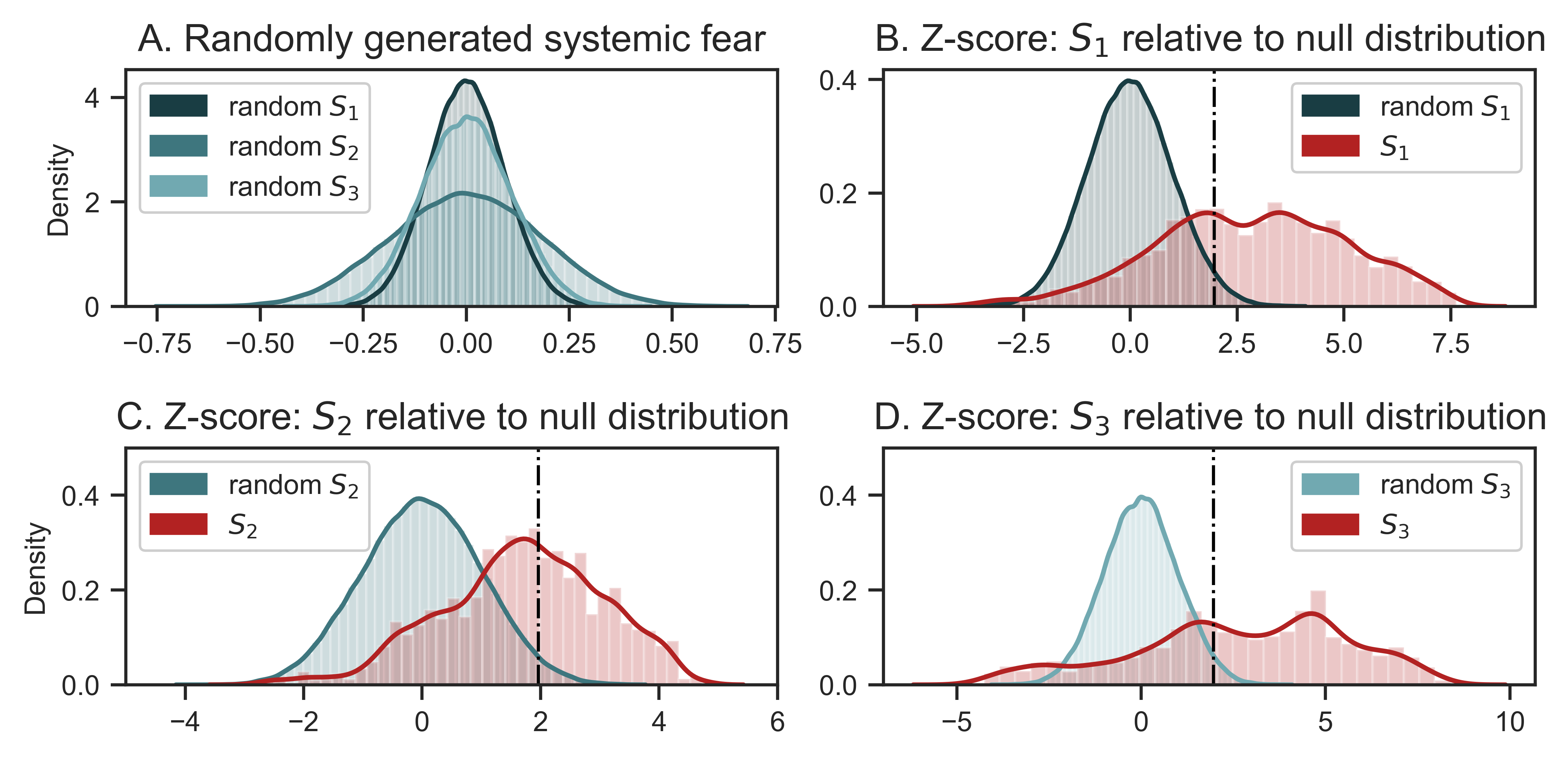
Figure 9: Distribution of systemic fear relative to the null-distribution
Note: This figure illustrates a thought experiment in which I compare the observed distribution of the systemic-fear index with a null distribution — the systemic-fear that would occur if prices and earnings are uncorrelated, random variables. Panel A shows the null distribution for each metric of systemic fear ( \footnotesize S_1 , \footnotesize S_2 and \footnotesize S_3 ). Panels C–D compare (for each different metric) the null distribution (blue) to the empirical distribution of systemic fear (red). I have displayed here the distributions in standardized, Z-score form. The dashed vertical lines indicate a Z-score of \footnotesize +1.96 , which corresponds to statistical significance at \footnotesize \alpha = 0.05 .
Source and methods: rolling correlations of random numbers are done with two series with 1 million observations. Z-scores calculated with the following results: null \footnotesize S_1~\text{mean} = 0 , \footnotesize \text{std} = 0.09 ; null \footnotesize S_2~\text{mean} = 0 , \footnotesize \text{std} = 0.18 ; null \footnotesize S_3~\text{mean} = 0 , \footnotesize \text{std} = 0.26 . See Table 2 for the creation of systemic-fear index \footnotesize S_1 , \footnotesize S_2 and \footnotesize S_3 . See Appendix for breakdown of data by country.
Panel A of Figure 9 shows the three null distributions of systemic fear — one for each different metric ( \footnotesize S_1 , \footnotesize S_2 and \footnotesize S_3 ). Each metric of systemic fear has a null distribution with a mean of zero. Yet notice that the standard deviations differ between metrics. Systemic-fear index \footnotesize S_1 (the measure used by Bichler and Nitzan as well as Baines and Hager) has the smallest standard deviation. This result indicates that the probability of systemic-fear index \footnotesize S_1 producing values above \footnotesize +0.25 and below \footnotesize -0.25 through randomness is low.
In Panels B, C, and D of Figure 9, I transform the respective measures of systemic fear into a Z-score (of the null distribution). I then plot the empirical distribution of systemic fear (red) against the null distribution (blue). This visualization indicates that, relative to the null distribution, there are both statistically insignificant and statistically significant measures of systemic fear. Empirical observations to the right of the dotted vertical line are above \footnotesize Z=+1.96 , which is statistically significant when \footnotesize \alpha = 0.05 . But we can also find systemic-fear observations with much higher levels of statistical significance.
Figure 10 plots time series of systemic fear (index \footnotesize S_1 ) for each country in my dataset. Shaded regions highlight periods when the observed value of systemic fear exceeds \footnotesize Z>4 (which corresponds to statistical significance at \footnotesize \alpha = 6.3 \times 10^{-5} ). Many observations after 2000 are shaded at this higher threshold for statistical significance. The statistical significance is also retained when at times systemic fear plateaus and decreases.10
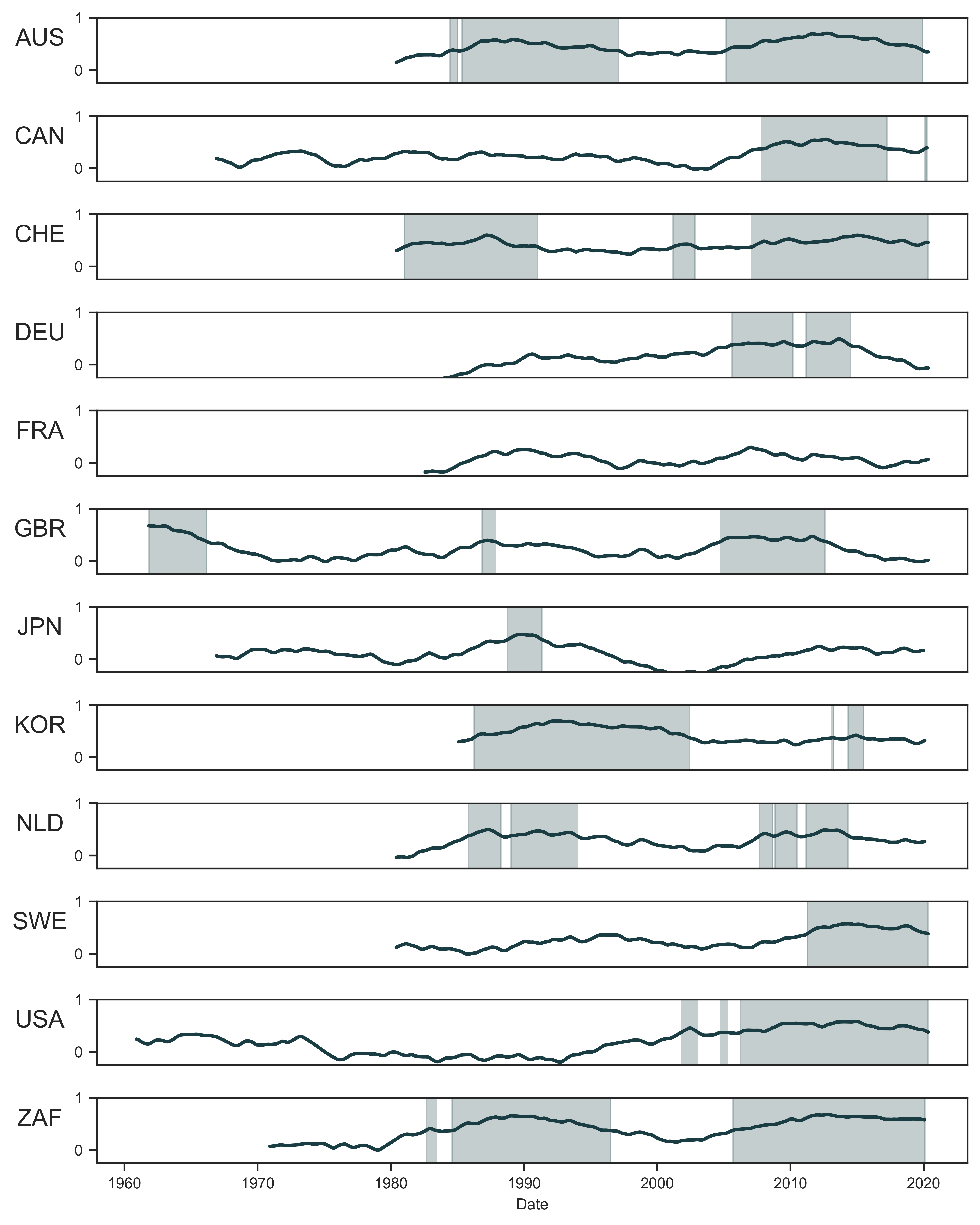
Figure 10: The statistical significance of systemic fear
Note: Each panel shows trends in the systemic fear (index \footnotesize S_1 ) for the countries in my dataset. Shaded regions indicate periods when the index is statistically significant (relative to the null distribution of systemic fear shown in Figure 9) at \footnotesize Z>4 .
Source and methods: See Figure 9.
4 Another look at systemic fear and capitalist power
I move now from revisiting Bichler and Nitzan’s concept of systemic fear to re-testing the connection between systemic fear and the power index. Recall that the power index is intended to measure the relative power of capitalists.
My expanded dataset reveals that countries such as Australia, Canada and Sweden have positive correlations between systemic fear (index \footnotesize S_1 ) and the power index ( \footnotesize P_1 ). In what follows, I explore the connection between capitalist power and systemic fear using new metrics of my own creation.
4.1 Testing different measures of systemic fear and capitalist power
In Section 2, I introduced 3 measures of systemic fear and 3 measures of the power index. (See Table 2 for their definitions.) So as not to distract the reader already familiar with the CasP model of the stock market, in the previous section I used the original measures of systemic fear ( \footnotesize S_1 ) and capitalist power ( \footnotesize P_1 ) proposed by Bichler and Nitzan. Moving forward, however, I will go beyond Bichler and Nitzan’s original metrics.
Why add more measures? Because the works of Bichler and Nitzan are a mixture of both empirical research and political-economic theory. If we retain the theoretical essences of systemic fear and the power index, we are free to experiment with their empirical measurement. Different metrics of systemic fear and capitalist power produce a spectrum of results, whereby we can identify what happens when parameters are changed.
Systemic fear, in particular, is ripe for experimentation. It measures fear that is expressed through a type of behavior — basing prices on past earnings — but it is unlikely that this behavior would be uniform across all capitalists in time and place. As when someone applies the forward-looking ritual of discounting a future income stream, the manner in which someone looks to past earnings could be affected by accounting methods, as well as by social and cultural variables such as business norms and subjectivity.
As a thought experiment, consider the 12-month correlation window in systemic-fear index \footnotesize S_1 — the metric devised by Bichler and Nitzan. What if that window was narrowed to 10 months? Or what if fearful capitalists were looking to the past earnings of 16 months, or even more? Political economists can debate the significance of such variations, but the original 12-month parameter is but one of many ways that capitalists, in a state of fear about the future, might base prices on past earnings.
Compared to the original metric \footnotesize S_1 , the systemic-fear measures \footnotesize S_2 and \footnotesize S_3 are sensitive to different changes in the correlation between prices and earnings. The systemic-fear measure \footnotesize S_2 is produced with a seasonal decomposition, whereby seasonality and residuals are removed from each time series.11 The systemic-fear measure \footnotesize S_3 is the product of 12-month differencing, which is a way to remove long-term trends from a time series. Without a long-term trend shared by the levels of prices and earnings, the result of a correlation window of 120 months is not necessarily positive and high.
With respect to the measure of capitalist power, the new power indices \footnotesize P_2 and \footnotesize P_3 experiment with different denominators in the ratio between stock-market prices and the income of the non-capitalist population. The original power index ( \footnotesize P_1 ) uses the average wage rate in the denominator. Power index \footnotesize P_2 uses income per capita. Power index \footnotesize P_3 uses GDP per capita.
Using Canada as an example, Figure 11 shows time series for the various measures of systemic fear and capitalist power. Note that the power indices are quite similar. That is because the various incomes in the denominator are all strongly correlated. With respect to systemic fear, the 3 metrics share a long-term trend. But over the short term, they diverge.
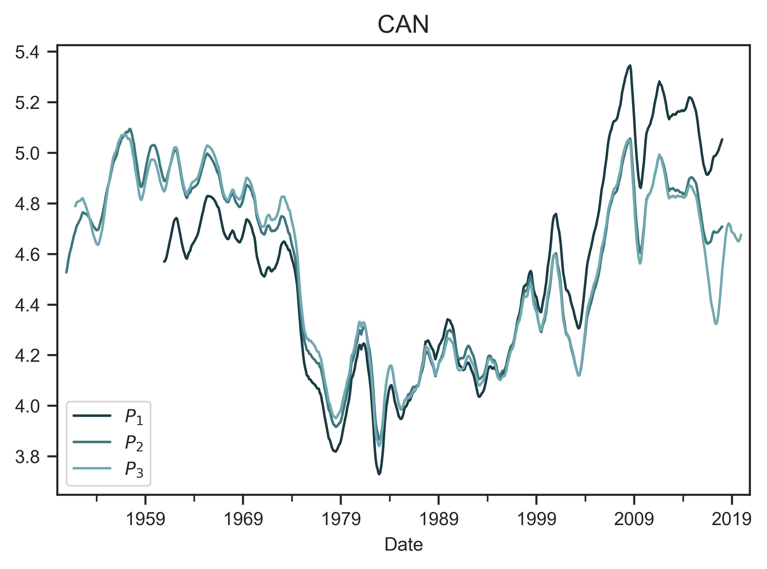
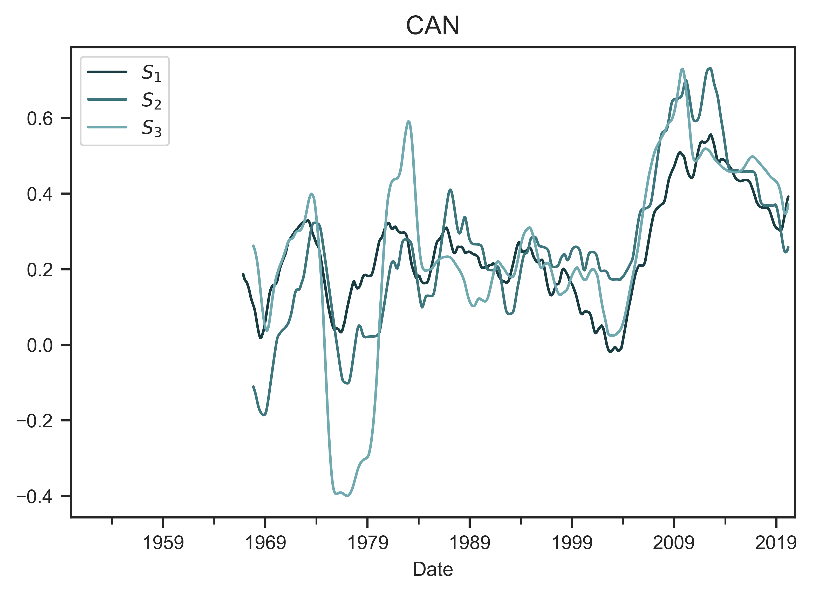
Figure 11: Indices of capitalist power and systemic fear in Canada
The top panel shows the three metrics of the power index in Canada ( \footnotesize P_1 , \footnotesize P_2 and \footnotesize P_3 ). The various indices share a similar trend, largely because their denominates are strongly correlated. The bottom panel shows the three metrics of the systemic fear in Canada ( \footnotesize S_1 , \footnotesize S_2 and \footnotesize S_3 ).
Source and methods: See Table 3 for the creation of power indices \footnotesize P_1 , \footnotesize P_2 and \footnotesize P_3 . See Table 2 for the creation of systemic-fear indices \footnotesize S_1 , \footnotesize S_2 and \footnotesize S_3 . See Appendix for breakdown of data by country.
With my expanded dataset of capitalist power and systemic fear, I ask the following questions:
-
Do countries have positive correlations between capitalist power and systemic fear, even if there is not a positive correlation between the original metrics ( \footnotesize S_1 and \footnotesize P_1 )?
-
If we use sample averages to estimate ‘expected’ values, is there a positive correlation between the ‘expected’ value of international capitalist power and international systemic fear?
4.2 Country-level correlations between systemic fear and capitalist power
To investigate the country-level correlation between systemic fear and capitalist power, Figure 12 summarizes all of the correlations between power indices ( \footnotesize P_i ) and systemic fear indices ( \footnotesize S_i ). Each row includes a systemic fear variable of a particular country. Each column is a specific power index. Boxes show the corresponding correlation between systemic fear and capitalist power. I have also used color to indicate the strength of the correlation. (Red indicates a stronger positive correlation. Blue indicates a stronger negative correlation.)
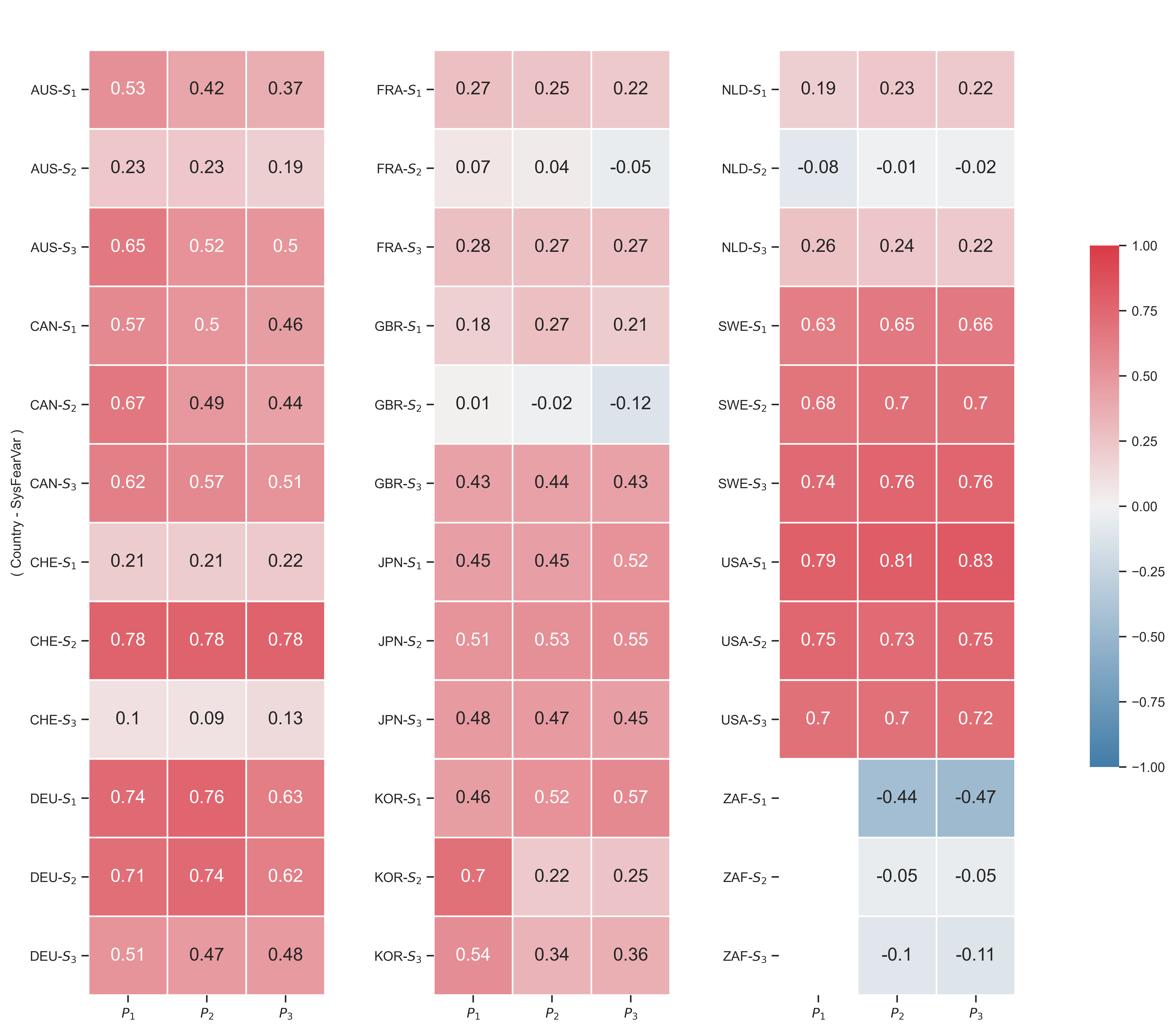
Figure 12: Country-level correlations between systemic fear and capitalist power
Note: Each box indicates the correlation (within a country) between a given measure of the power index (horizontal axis) and a given measure of systemic fear (vertical axis). Color indicates the strength of the correlation. (Red indicates a stronger positive correlation. Blue indicates a stronger negative correlation.)
Source and methods: See Table 2 for the creation of systemic-fear indices \footnotesize S_1 , \footnotesize S_2 and \footnotesize S_3 . See Table 3 for the creation of power indices \footnotesize P_1 , \footnotesize P_2 and \footnotesize P_3 . See Appendix for breakdown of data by country. See Figure 16 for p-values of each correlation.
In Figure 12, there are three notable results. First, a few countries (the United States, Germany and Sweden), show positive correlations across all nine combinations of indicators. Second, there are some countries (Switzerland, Australia and South Korea) that have at least one strong positive relationship between power and systemic fear. Third, France, the Netherlands and the United Kingdom have a few positive correlations. But more interestingly, their correlations are positive/negative in a similar way: \footnotesize S_1 is positive, \footnotesize S_2 is close to zero, and \footnotesize S_3 is positive and slightly stronger than \footnotesize S_1 .
First discovered by Baines and Hager, I reconfirm here that the correlation between capitalist power and systemic fear varies across countries. In their summary of findings, Baines and Hager conclude that Germany is the only country in their dataset that has similar results to the United States. We can now add Sweden (and possibly Australia, Canada, South Korea and Switzerland) to the list of countries in which capitalist power positively correlates with systemic fear.
My results also reveal that additional countries (such the Netherlands and South Africa) are different from the United States. In the case of South Africa, the partial results (due to missing data) suggest that it might have a moderate negative relationship between power and systemic fear — a quality that is both unique among countries in this dataset, and unexpected by the CasP model of the stock market.
4.3 International systemic fear and capitalist power
Moving forward, the international evidence for a positive relation between capitalist power and systemic fear might not be as weak as Baines and Hager claim. Even when the two variables diverge at the national level, their international averages remain correlated.
As shown in Figures 5 and 6, the systemic fear of many countries move together. These strong correlations cause average systemic fear (the unweighted mean across my sample of countries) to fluctuate coherently. In particular, note that since the late 1970s, average systemic fear has been rising. Such behavior suggests that systemic fear is indeed ‘systemic’ across countries. (If the United States was exceptional in having rising systemic fear, it is unlikely that an unweighted average with 11 other countries would rise.)
With this result in mind, I propose an international CasP model of the stock market in which I treat capitalist power and systemic fear probabilistically. If both capitalist power and systemic fear are ‘systemic’ (and if Bichler and Nitzan’s core hypothesis is correct), then ‘expected’ international capitalist power should correlate with ‘expected’ international systemic fear.
In mathematical terms, this ‘expected’ international value is revealed by the average (the sample mean) across my sample of countries.12 Therefore, I propose we study the relation between international capitalist power and international systemic fear by looking at their ‘expected’ value — their averages across countries.
Having already calculated averages of systemic fear (Figure 4), I do the same for the power index. Figure 13 plots the cross-country average of capitalist power. Each panel shows a different metric ( \footnotesize P_1 , \footnotesize P_2 and \footnotesize P_3 ). The blue line indicates the sample average. The shaded region indicates the standard deviation across countries. Similar to what we saw with systemic fear, I find that the international average of capitalist power has been rising since 1980.13
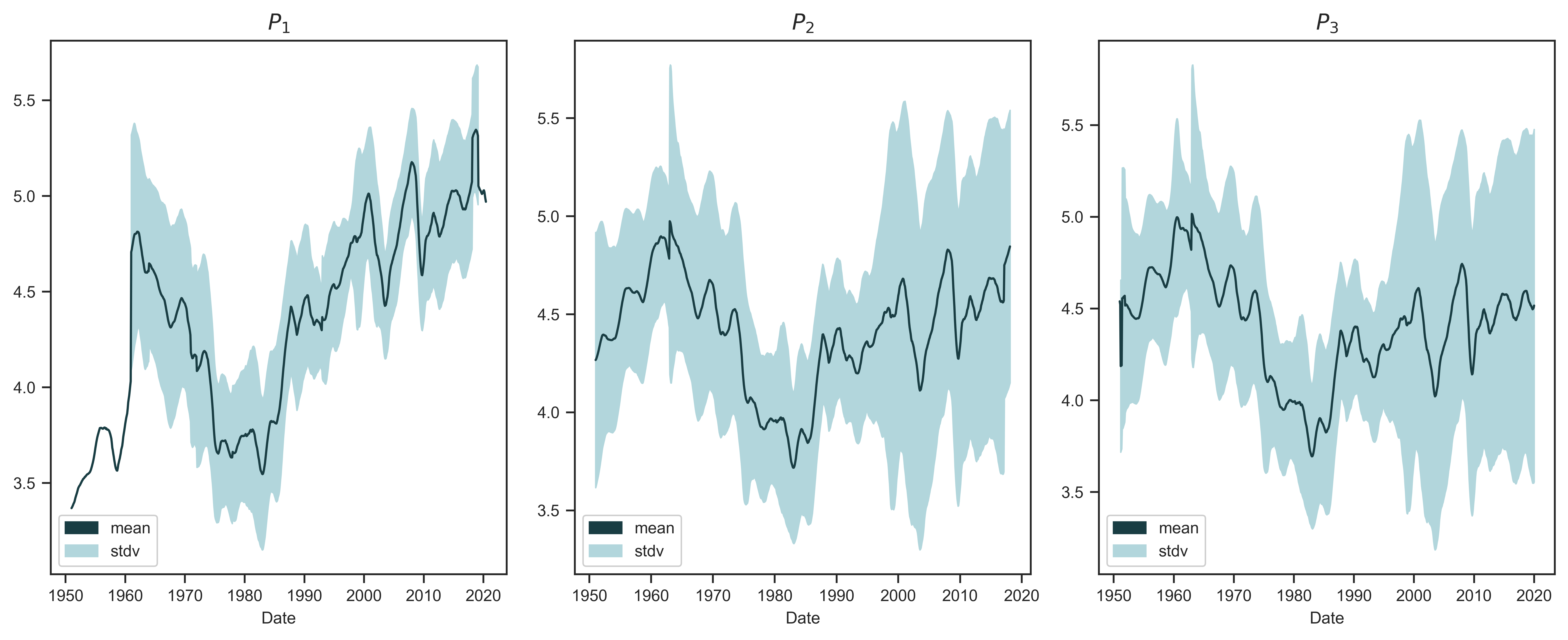
Figure 13: International averages of capitalist power
Note: Each panel shows a different measure of capitalist power (power indices \footnotesize P_1 , \footnotesize P_2 and \footnotesize P_3 ). To produce the trend line in each panel, I take the unweighted average of the power index across the 12 countries in my sample. The solid line indicates the average across the 12 countries observed here. The shaded region indicates the standard deviation.
Source and methods: See Table 3 for the creation of power indices \footnotesize P_1 , \footnotesize P_2 and \footnotesize P_3 . See Appendix for breakdown of data by country.
Figure 14 shows a three-by-three grid of ‘expected’ systemic fear plotted against ‘expected’ capitalist power. Although the relationships vary, all variable combinations are positively correlated. Moreover, specific combinations yield strong correlations. The first column of panels suggests that the variance of ‘expected’ capitalist power \footnotesize \overline{P_1} can explain between 48% and 61% of the variance of ‘expected’ systemic fear. This result suggests that in probabilistic terms, there is a strong international relation between capitalist power and systemic fear.
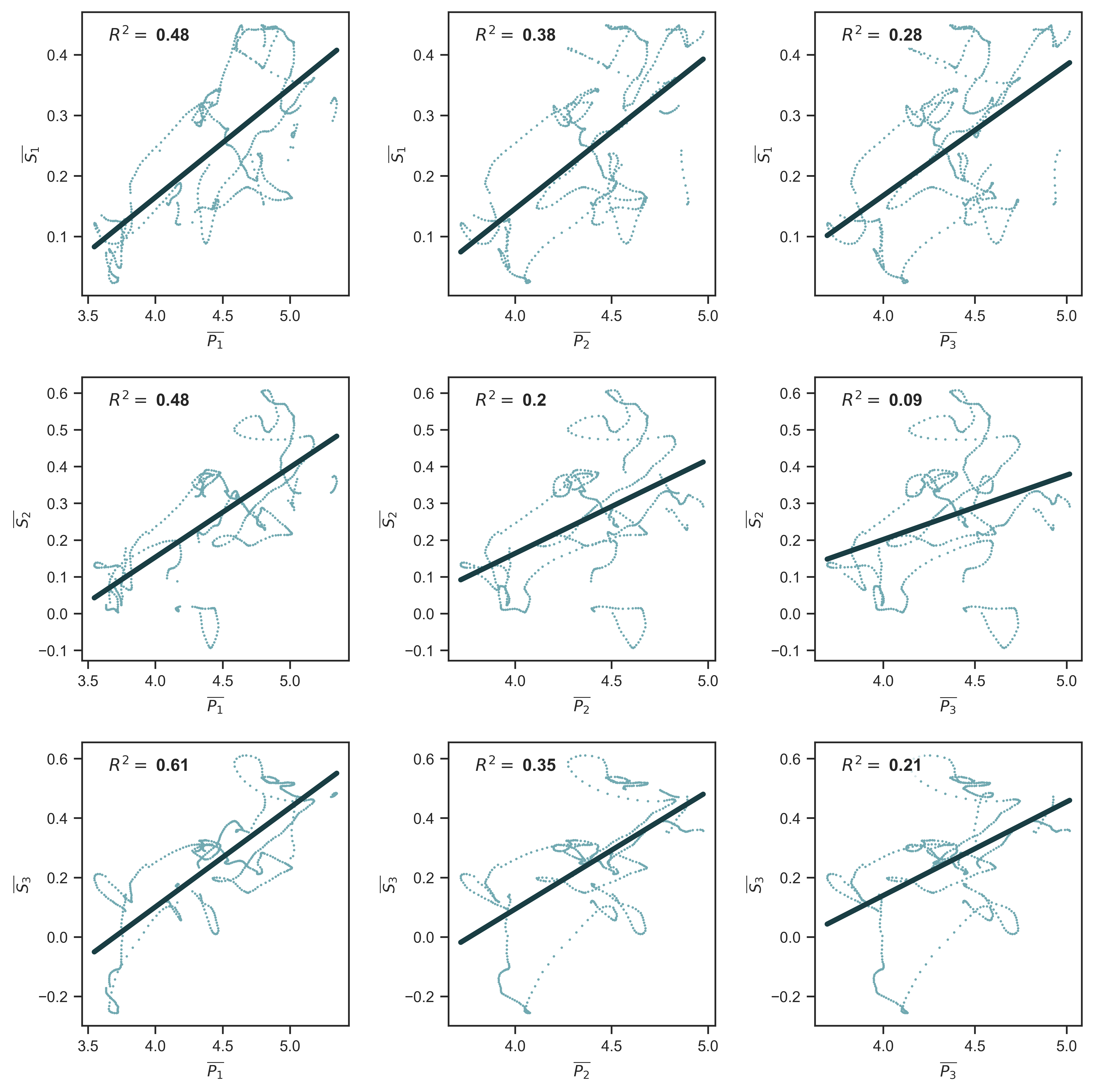
Figure 14: Relation between ‘expected’ systemic fear and ‘expected’ capitalist power for all combinations of indices
Note: Each panel shows a different pairing of systemic-fear indices \footnotesize S_1 , \footnotesize S_2 and \footnotesize S_3 and power indices \footnotesize P_1 , \footnotesize P_2 and \footnotesize P_3 . I plot here the correlation between the monthly sample means of each metric — the monthly average across my sample of countries. For a visualization of the cross-country mean of systemic fear, see Figure 4. For a visualization of the cross-country mean of the power index, see Figure 13.
Source and methods: See Table 2 for the creation of systemic-fear indices \footnotesize S_1 , \footnotesize S_2 and \footnotesize S_3 . See Table 3 for the creation of power indices \footnotesize P_1 , \footnotesize P_2 and \footnotesize P_3 . See Appendix for breakdown of data by country.
5 Conclusion
The relation between systemic fear and capitalist power is a key aspect of the capital-as-power (CasP) model of the stock market. But it is not the only component. In their test of the CasP model, Baines and Hager also look for an inverse relation between the power index and employment growth — a relation they label ‘strategic sabotage’ in reference to Bichler and Nitzan’s use of Thorstein Veblen’s term (Nitzan & Bichler, 2009; Veblen, 2004). Baines and Hager also investigate how employment growth relates to the yield of 10-year government bonds — a relation they call the ‘CasP Policy Cycle’ (Baines & Hager, 2020, p. 124).
The sum of their results leads Baines and Hager to conclude that the CasP model of the stock market is at odds with the evidence. Bichler and Nitzan’s US results do not seem to hold in other countries. One option would be to . But doing so lessens our ability to explain the behavior of other major stock markets. Baines and Hager therefore conclude:
The main lesson from our analysis here is that the evolution of the stock market in other advanced capitalist countries cannot simply be read off from the US experience.
(Baines & Hager, 2020, p. 137)
I contend that the concept of systemic fear is more promising than Baines and Hager believe. In fact, the closer we look at systemic fear, the more it seems to support, rather than undermine, Baines and Hager’s goal of explaining (Baines & Hager, 2020, p. 137).
Among the 12 countries studied here, there is evidence for global unevenness and national diversity in systemic fear. But this national diversity is not so great as to render systemic fear a meaningless concept. Despite national differences, international systemic fear has risen ‘systemically’. And despite national differences, international ‘expected’ systemic fear correlates positively with international ‘expected’ capitalist power.
Going forward, we should certainly not ignore the negative correlations between systemic fear and capitalist power. For example, my results for Great Britain are similar to those of Baines and Hager. Further research is needed to explain why certain countries — countries like Great Britain, France, the Netherlands and South Africa — are different from those in which systemic fear and capitalist power correlate positively.
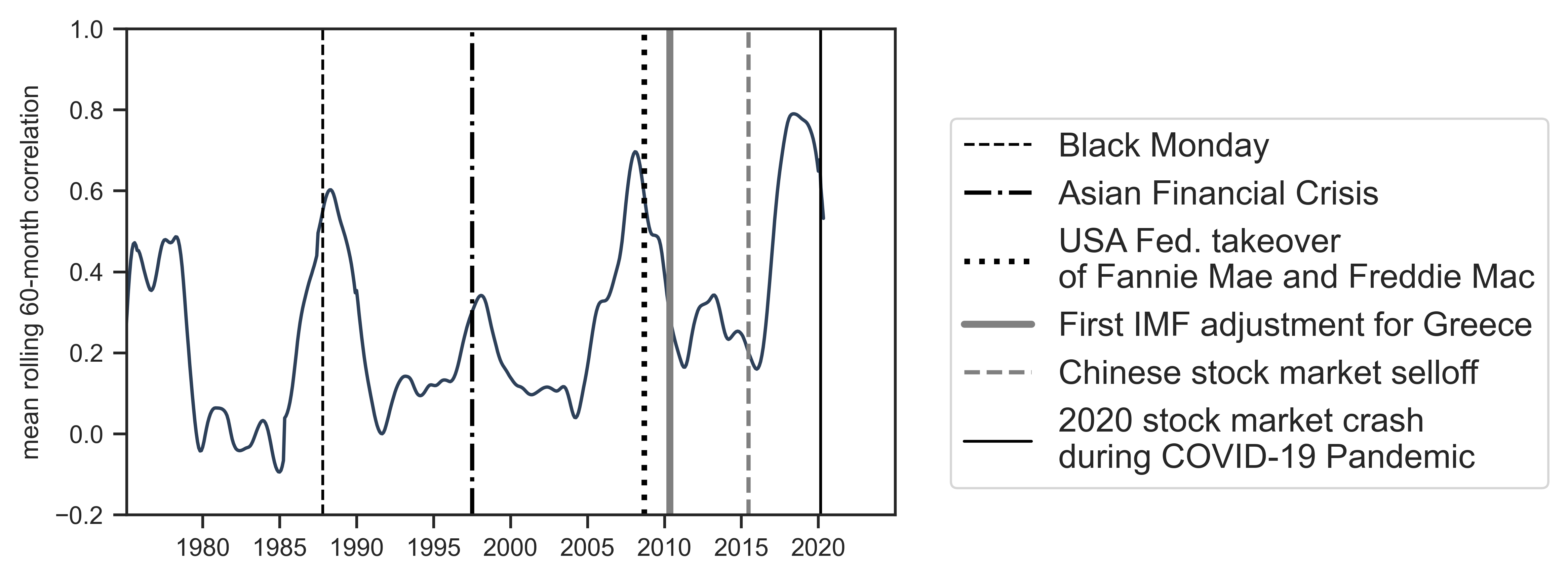
Figure 15: Political-economic crisis and the co-experience of systemic fear
Note: This figure plots the average 60-month correlation of systemic-fear index \footnotesize S_1 across all countries in my dataset. (See Figure 6 for the individual correlations.) When the cross-correlation rises, it indicates that countries co-experience systemic fear. This co-experience seems to increase during periods of political-economic crises (vertical lines).
Source and methods: See Figure 6 for the 60-month rolling correlation of each country’s \footnotesize S_1 with other countries in the dataset. Dates of financial events were taken from Wikipedia.
In addition to diving deeper into the negative correlations, there is opportunity to build a richer understanding of when advanced capitalist countries co-experience systemic fear. On that front, Figure 15 plots the average correlation of systemic-fear index \footnotesize S_1 across all pairings of countries in my dataset. When this average rises, it suggests that these countries are co-experiencing systemic fear. Notably, peaks in the country-country correlation occur near or during some of the major political-economic crises of the past forty years (plotted as vertical lines). It seems unlikely that this alignment is a coincidence.
As of this writing, we are living through another peak in the co-experience of systemic fear. The significance of this pattern is worth investigating, and warrants taking a closer look at the concept of systemic fear.
Acknowledgements
I would like to thank the two anonymous reviewers for their thorough comments. I also would like to thank Joseph Baines, Blair Fix, Sandy Hager, and Jonathan Nitzan. They read this paper when it was a working paper and encouraged me to publish my ideas on the CasP model of the stock market.
Appendix: Data sources and supplementary data
Tables 5–10 provide country breakdowns for the data in this paper. The majority of the data was accessed through Global Financial Data (indicated in the title of each table). The exception is Table 8, which uses a variety of sources.
Figure 16 summarizes the statistical significance of the cross-country correlation between power indices and systemic fear.
Table 5: Data sources for Composite Index Prices (from Global Financial Data)
| Country | Ticker | Frequency | Start Date | End Date |
|---|---|---|---|---|
| Australia | _AORDD | Monthly | 01/31/1950 | 04/30/2020 |
| Canada | _GSPTSED | Monthly | 01/31/1950 | 04/30/2020 |
| France | _CACTD | Monthly | 01/31/1950 | 04/30/2020 |
| Germany | _CXKXD | Monthly | 01/31/1950 | 04/30/2020 |
| Japan | _TOPXD | Monthly | 01/31/1950 | 04/30/2020 |
| Netherlands | _AAXD | Monthly | 01/31/1950 | 04/30/2020 |
| South Africa | _JALSHD | Monthly | 01/31/1950 | 04/30/2020 |
| South Korea | _KS11D | Monthly | 01/31/1962 | 04/30/2020 |
| Sweden | _OMXSPID | Monthly | 01/31/1950 | 04/30/2020 |
| Switzerland | _SPIXD | Monthly | 01/31/1950 | 04/30/2020 |
| United Kingdom | _FTASD | Monthly | 01/31/1950 | 04/30/2020 |
| United States | _SPXD | Monthly | 01/31/1950 | 04/30/2020 |
Table 6: Data sources for price-earnings ratios (from Global Financial Data)
| Country | Ticker | Frequency | Start Date | End Date |
|---|---|---|---|---|
| Australia | SYAUSPM | Monthly | 07/31/1969 | 04/30/2020 |
| Canada | SYCANPTM | Monthly | 01/31/1956 | 03/31/2020 |
| France | SYFRAPM | Monthly | 09/30/1971 | 04/30/2020 |
| Germany | SYDEUPM | Monthly | 07/31/1969 | 04/30/2020 |
| Japan | SYJPNPTM | Monthly | 01/31/1956 | 12/31/2019 |
| Netherlands | SYNLDPM | Monthly | 07/31/1969 | 01/31/2020 |
| South Africa | SYZAFPM | Monthly | 01/31/1960 | 01/31/2020 |
| South Korea | SYKORPM | Monthly | 03/31/1974 | 01/31/2020 |
| Sweden | SYSWEPM | Monthly | 07/31/1969 | 04/30/2020 |
| Switzerland | SYCHEPM | Monthly | 07/31/1969 | 04/30/2020 |
| United Kingdom | _PFTASD | Monthly | 12/31/1950 | 04/30/2020 |
| United States | SYUSAPM | Monthly | 01/31/1950 | 04/30/2020 |
Table 7: Data sources for nominal GDP per capita (from Global Financial Data)
| Country | GDP Ticker | GDP Frequency | Pop. Ticker | Start Date | End Date |
|---|---|---|---|---|---|
| Australia | GDPAUS | Annual until 1959; trimonthly after | POPAUS | 06/30/1950 | 12/31/2019 |
| Canada | GDPCAN | Annual until 1957; trimonthly after | POPCAN | 12/31/1950 | 12/31/2019 |
| France | GDPFRA | Annual until 1966; trimonthly after | POPFRA | 12/31/1950 | 12/31/2019 |
| Germany | GDPDEU | Annual until 1961; trimonthly after | POPDEU | 12/31/1950 | 12/31/2019 |
| Japan | GDPJPN | Annual until 1981; trimonthly after | POPJPN | 12/31/1950 | 12/31/2019 |
| Netherlands | GDPNLD | Annual until 1978; trimonthly after | POPNLD | 12/31/1950 | 12/31/2019 |
| South Africa | GDPZAF | Annual until 1960; trimonthly after | POPZAF | 12/31/1950 | 12/31/2019 |
| South Korea | GDPKOR | Annual until 1961; trimonthly after | POPKOR | 12/31/1953 | 12/31/2019 |
| Sweden | GDPSWE | Annual until 1981; trimonthly after | POPSWE | 12/31/1950 | 12/31/2019 |
| Switzerland | GDPCHE | Annual until 1971; trimonthly after | POPCHE | 12/31/1950 | 12/31/2019 |
| United Kingdom | GDPGBR | Annual until 1956; trimonthly after | POPGBR | 12/31/1950 | 12/31/2019 |
| United States | GDPUSA | Trimonthly | POPUSA | 03/31/1950 | 12/31/2019 |
Table 8: Data sources for wage rates (2015 \footnotesize = 100 )
| Country | Ticker | Category | Source | Frequency | Start Date | End Date |
|---|---|---|---|---|---|---|
| Australia | LCWRTT01AUA661N | All Activities | OECD (via FRED) | Annual | 1977 | 2018 |
| Canada | LCEAMN01CAA661N | Manufacturing | OECD (via FRED) | Annual | 1960 | 2018 |
| France | LCWRMN01FRA661N | Manufacturing | OECD (via FRED) | Annual | 1960 | 2018 |
| Germany | LCEAMN01DEA661N | Manufacturing | OECD (via FRED) | Annual | 1960 | 2018 |
| Japan | LCEAMN01JPA661S | Manufacturing | OECD (via FRED) | Annual | 1960 | 2018 |
| Netherlands | LCWRMN01NLM661N | Manufacturing | OECD (via FRED) | Annual | 1960 | 2018 |
| South Africa | South Korea LCEAMN01KRA661S Manufacturing OECD (via FRED) Annual 1992 2018 | |||||
| Sweden | LCEAMN01SEA661N | Manufacturing | OECD (via FRED) | Annual | 1971 | 2018 |
| Switzerland | T 39 | All Activities | Swiss Statistical Office | Annual | 1950 | 2018 |
| United Kingdom | LCEAMN01GBA661S | Manufacturing | OECD (via FRED) | Annual | 1963 | 2018 |
| United States | LCEAMN01USA661N | Manufacturing | OECD (via FRED) | Annual | 1960 | 2018 |
Table 9: Data sources for Buffet Indicator (Market cap / GDP) (from Global Financial Data)
| Country | Ticker | Frequency | Start Date | End Date |
|---|---|---|---|---|
| Australia | SCAUSMPC | Annual | 12/31/1950 | 12/31/2019 |
| Canada | SCCANMPC | Annual until 1951; monthly after | 12/31/1950 | 12/31/2019 |
| France | SCFRAMPC | Annual until 1955; monthly after | 12/31/1950 | 02/29/2020 |
| Germany | SCDEUMPC | Annual until 1960; trimonthly until 1968; monthly after | 12/31/1950 | 01/31/2020 |
| Japan | SCJPNMPC | Monthly | 01/31/1950 | 01/31/2020 |
| Netherlands | SCNLDMPC | Annual until 1991; monthly after | 12/31/1950 | 02/29/2020 |
| South Africa | SCZAFMPC | Monthly | 01/31/1950 | 01/31/2020 |
| South Korea | SCKORMPC | Annual until 1978; monthly after | 12/31/1961 | 01/31/2020 |
| Sweden | SCSWEMPC | Annual until 1991; monthly after | 12/31/1950 | 02/29/2020 |
| Switzerland | SCCHEMPC | Annual until 1990; montly after 11/30/1990 | 12/31/1950 | 01/31/2020 |
| United Kingdom | SCGBRMPC | Annual until 1995; monthly after | 03/31/1952 | 01/31/2020 |
| United States | SCUSAMPC | Monthly | 01/31/1950 | 01/31/2020 |
Table 10: Data sources for CAPE3 ratio (from Global Financial Data)
| Country | Ticker | Frequency | Start Date | End Date |
|---|---|---|---|---|
| Australia | SYAUSCAPE3M | Monthly | 06/30/1972 | 12/31/2019 |
| Canada | SYCANCAPE3M | Monthly | 12/31/1958 | 12/31/2019 |
| France | SYFRACAPE3M | Monthly | 08/31/1974 | 02/29/2020 |
| Germany | SYGBRCAPE3M | Monthly | 06/30/1972 | 04/30/2020 |
| Japan | SYJPNCAPE3M | Monthly | 12/31/1958 | 04/30/2020 |
| Netherlands | SYNLDCAPE3M | Monthly | 06/30/1972 | 04/30/2020 |
| South Africa | SYZAFCAPE3M | Monthly | 12/31/1962 | 04/30/2020 |
| South Korea | SYKORCAPE3M | Monthly | 02/28/1977 | 04/30/2020 |
| Sweden | SYSWECAPE3M | Monthly | 06/30/1972 | 04/30/2020 |
| Switzerland | SYCHECAPE3M | Monthly | 06/30/1972 | 01/31/2020 |
| United Kingdom | SYGBRCAPE3M | Annual until 1961; monthly after 04/30/1962 | 12/31/1950 | 01/31/2020 |
| United States | SYUSACAPE3M | Monthly | 01/31/1950 | 04/30/2020 |
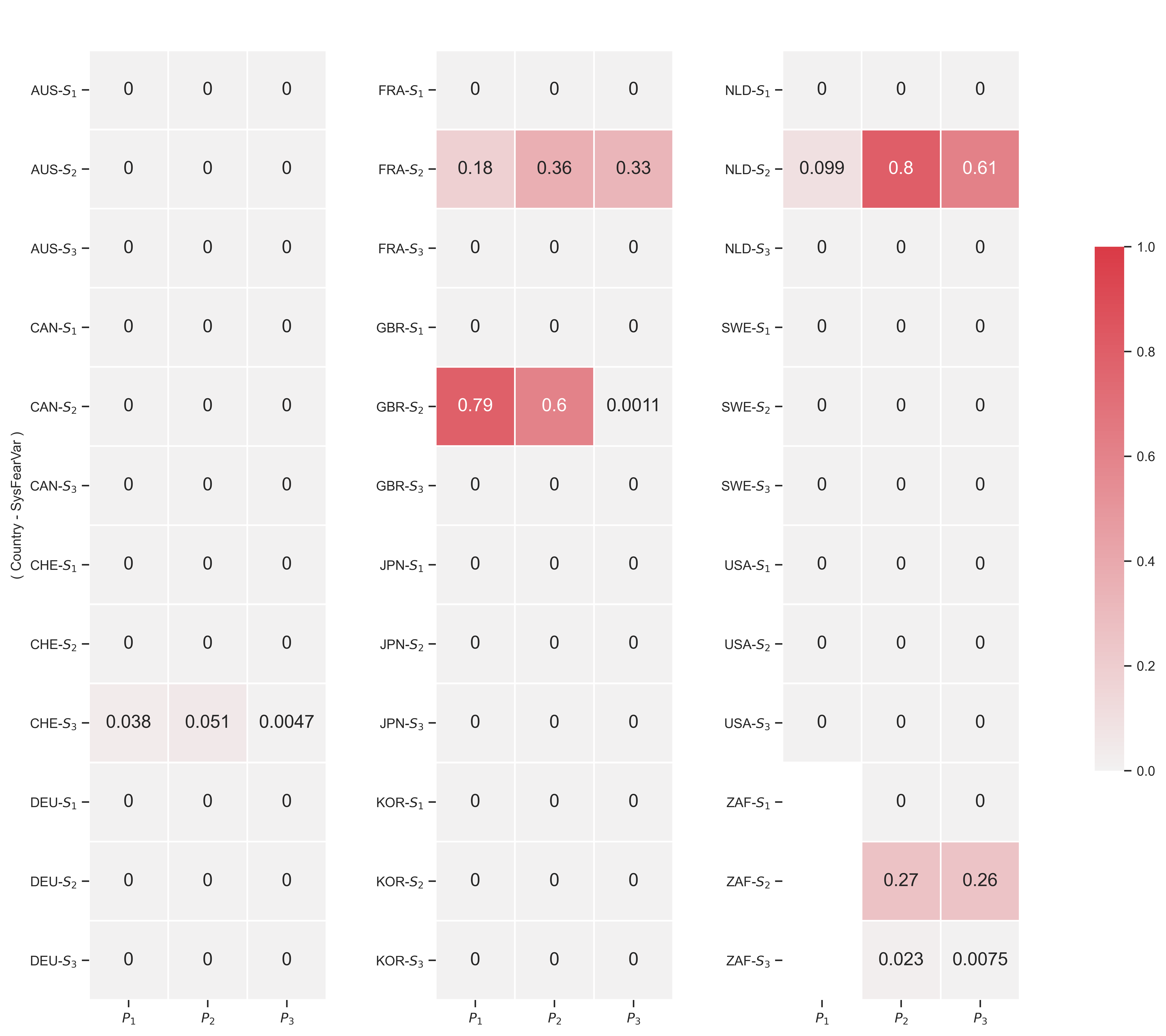
Figure 16: P-values for the country-level correlations between capitalist power and systemic fear
Note: Each box shows the \footnotesize p -value for the correlation (in the given country) between the given metric of capitalist power (either \footnotesize P_1 , \footnotesize P_2 and \footnotesize P_3 ) and the given metric of systemic fear (either \footnotesize S_1 , \footnotesize S_2 and \footnotesize S_3 ). \footnotesize P -values below 0.00005 are rounded down to 0. The associated correlation coefficients are shown in Figure 12.
Notes
James McMahon currently teaches at the University of Toronto, Canada. His main research interests are the Hollywood film business, social theories of mass culture and political economic theory.
-
Readers unfamiliar with how Bichler and Nitzan use the terms ‘power’ and ‘accumulation’ should start with (Nitzan & Bichler, 2009). Their methods are easy to understand but the reader is asked to pay special attention to the theoretical assumptions that are rejected. For example, in their paper that presents a CasP model of the stock market, they reject the idea that there can be mismatches between nominal financial prices and real economic units of production and consumption (Bichler & Nitzan, 2016).↩
-
They do find a tight positive correlation for France, but the time-span of data (1999-2017) is shorter than what they have for Germany (1983-2017).↩
-
(Kliman, 2011) likewise critiques Bichler and Nitzan’s model without exploring alternative reasons for apparent failures.↩
-
An investigation of the U-turn from declining systemic fear in the 1960s to rising systemic fear in the 1980s is warranted. A quickly-made hypothesis would identify the cause to be the rise of a neo-liberal political economy.↩
-
Thanks go to an anonymous reviewer for the revision of this paragraph. If any errors remain, they are my own.↩
-
Evidence of this outcome would support Baines and Hager’s argument.↩
-
Ultimately, one’s threshold for empirical difference will impact how one sees a strong network of relations in Figure 5. Further research will be needed to explore the network of relations in rising or falling systemic fear.↩
-
Summarizing their notion of ‘confidence in obedience’, Bichler and Nitzan write:
[T]he only reason for capitalists to buy stocks and in so doing bid up the stock price/wage ratio is that they expect this ratio to rise even further. And the fact that they believe that this ratio will go up attests to their confidence in obedience — the confidence that the underlying population will not expropriate them and that the system as a whole will not fail them. In this sense, our power index offers an objective measure of capitalist confidence — at least on the outside.
(Bichler & Nitzan, 2016, p. 142) -
(Kliman, 2011) was one of the first to critique Bichler and Nitzan’s concept of systemic fear. Kliman makes it very clear that he thinks it is impossible for systemic fear to be a meaningful concept because the evidence is showing a rise of systemic fear in two periods, June 1953–August 1962 and August 1962–December 1973. Lest I be perceived to be exaggerating Kliman’s argument that systemic fear cannot be high at particular points in time, here is a key quotation in full:
But B&N haven’t merely gotten their facts wrong. Because their facts are wrong, so is their paper’s key claim that we can infer that investors are gripped by when the relationship between current profits and equity prices is strong and positive. They tell us that the two periods in which systemic fear prevailed were two periods of acute crisis, the Great Depression and the 2000s. If a strongly positive correlation between current profits and share prices were another exceptional feature of these periods of crisis, then the notion that we can infer the existence of systemic fear from the positive correlation might be plausible. But the 1930s and 2000s were not exceptional in that respect, as we have seen. And the other two strongly positive-correlation periods, which run from the early 1950s through the early 1970s, cannot plausibly be characterized as a time of systemic fear. On the contrary, that era was the so-called golden age of capitalism. So a strongly positive correlation between current profits and equity prices does not allow us to infer the existence of systemic fear.
(Kliman, 2011, p. 64, italics in original)In response to Kliman, Bichler and Nitzan acknowledged their factual error, analyzed the significance of a high correlation of prices and earnings occurring between the 1950s and the 1970s, and produced an alternative method for measuring systemic fear (Bichler & Nitzan, 2011, 2016). To my knowledge, Kliman has not explained if his views on the concept would change if Bichler and Nitzan got their facts ‘right’.↩
-
There are opportunities to investigate the periodicity of a country’s high systemic fear. For example, South Africa’s first wave of high systemic fear occurred in the final years of Apartheid. The timing of this wave also complements the analysis of (Nitzan & Bichler, 2001), who argue that the collapse of the Apartheid regime coincides with changes to how dominant South African firms achieved differential accumulation.↩
-
I used the
seasonal_decomposefunction from the Python librarystatsmodels.tsa.seasonal.↩ -
The sample mean is an estimate of the expected population mean, and therefore serves as an estimate of the ‘expected’ average for a random sample drawn from the population.↩
-
Of the three measures of the power index, measure \footnotesize P_1 increases the most from 1950 to 2020 and from 1980 to 2020. That is because compared to the wage rate (the denominator in \footnotesize P_1 ), the denominators in \footnotesize P_2 (average income per capita) and \footnotesize P_3 (nominal GDP per capita) are prone to rise when inequality increases. (Growing income among top earners pulls up the average income.)↩
References
Baines, J., & Hager, S. B. (2020). Financial crisis, inequality, and capitalist diversity: A critique of the capital as power model of the stock market. New Political Economy, 25(1), 122–139. https://doi.org/10.1080/13563467.2018.1562434
Bichler, S., & Nitzan, J. (2011). Kilman on Systemic Fear: A Rejoinder. Journal of Critical Globalization Studies, (4), 93–118.
Bichler, S., & Nitzan, J. (2016). A CasP model of the stock market. Real-World Economics Review, 77, 118–154.
Buffett, W. (2001). Warren Buffett on the Stock Market. Fortune, 144(12), 80–94. http://search.ebscohost.com.myaccess.library.utoronto.ca/login.aspx?direct=true&db=buh&AN=5594803&site=ehost-live
Castoriadis, C. (1998). The Imaginary Institution of Society (K. Blamey, Trans.). Cambridge, Massachusetts: The MIT Press.
Hume, D. (1985). A Treatise of Human Nature (E. C. Mossner, Ed.). Penguin Books.
Kliman, A. (2011). Value and Crisis: Bichler and Nitzan versus Marx. Journal of Critical Globalization Studies, (4), 61–92.
Knight, F. H. (1921). Risk, uncertainty and profit. Boston, MA: Houghton Mifflin Company.
MSCI. (2020). MSCI World Index (USD) [Factsheet]. MSCI website: https://www.msci.com/documents/10199/149ed7bc-316e-4b4c-8ea4-43fcb5bd6523
Nitzan, J., & Bichler, S. (2001). Going Global: Differential Accumulation and the Great U-turn in South Africa and Israel. Review of Radical Political Economics, 33(1), 21–55.
Nitzan, J., & Bichler, S. (2009). Capital as Power: A Study of Order and Creorder. New York: Routledge.
OECD. (2020). Business confidence index (bci) (indicator). https://doi.org/10.1787/3092dc4f-en
Shiller, R. J. (2005). Irrational exuberance: (Second edition). Princeton University Press.
Veblen, T. (2004). Absentee Ownership: Business Enterprise in Recent Times: The Case of America. New Brunswick, NJ: Transaction Publishers.